Systems Biology in Biomarker Discovery: Integrating Multi-Omics and Computational Approaches for Precision Medicine

Abstract

This article provides a comprehensive overview of how systems biology approaches are revolutionizing biomarker discovery for researchers, scientists, and drug development professionals. It explores the foundational principles of moving beyond single-molecule biomarkers to integrated multi-omics panels, details cutting-edge computational methodologies including machine learning and dynamic selection algorithms, addresses key challenges in data integration and validation, and examines frameworks for ensuring clinical translatability. By synthesizing recent technological advancements and current research trends, this content serves as both an educational resource and practical guide for implementing systems biology strategies to identify robust, clinically relevant biomarkers across various disease states, ultimately accelerating the development of personalized medicine.

From Single Molecules to Integrated Systems: The New Paradigm in Biomarker Science

In modern biomedical research, a biomarker is defined as "a defined characteristic that is measured as an indicator of normal biological processes, pathogenic processes, or responses to an exposure or intervention" [1]. The emergence of systems biology has fundamentally transformed biomarker discovery from a traditional reductionist approach focused on single molecules to a holistic discipline that considers the complex interactions between biological components [2]. This paradigm shift recognizes that diseases arise from perturbations across interconnected networks of genes, proteins, and metabolites rather than isolated molecular defects [3].

Systems biology approaches leverage high-throughput technologies and computational analytics to integrate multi-omics data, providing unprecedented insights into disease mechanisms [4]. This integrative framework has enabled the identification of biomarker signatures that capture the complexity of diseases more effectively than single biomarkers, leading to improved diagnostic accuracy and treatment personalization [5]. The application of systems biology principles has proven particularly valuable for understanding complex diseases such as cancer, neurological disorders, and adverse drug reactions, where multiple biological pathways are involved simultaneously [3] [2].

Table: Classification of Biomarkers by Clinical Application

Biomarker Type	Primary Function	Clinical Utility	Examples
Diagnostic	Detect or confirm disease presence	Early disease detection, differential diagnosis	PSA (prostate cancer), troponin (myocardial infarction) [1]
Prognostic	Predict disease course and outcome	Inform treatment intensity, patient counseling	Oncotype DX (breast cancer recurrence) [1]
Predictive	Identify likely treatment responders	Guide therapy selection, optimize outcomes	HER2 status (trastuzumab response) [1]
Pharmacodynamic	Show biological drug activity	Monitor treatment response, guide dosing	Blood pressure (antihypertensives), viral load (antivirals) [1]
Safety	Detect potential adverse effects	Prevent treatment complications, ensure safety	Liver function tests, kidney function markers [1]

Biomarker Types and Molecular Characteristics

Biomarkers encompass diverse molecular classes that provide complementary biological information. Each biomarker type reflects different aspects of physiological or pathological processes, with varying origins, detection technologies, and clinical applications [4].

Genetic biomarkers include DNA sequence variants, single nucleotide polymorphisms (SNPs), and gene expression regulatory changes detectable through whole genome sequencing, PCR, and SNP arrays. These biomarkers facilitate genetic disease risk assessment, drug target screening, and tumor subtyping [4]. Epigenetic biomarkers comprise DNA methylation patterns, histone modifications, and chromatin remodeling events measured via methylation arrays and ChIP-seq technologies, offering insights into environmental exposure assessments and early cancer diagnosis [4].

Transcriptomic biomarkers involve mRNA expression profiles, non-coding RNAs, and alternative splicing events analyzed through RNA-seq and microarrays, enabling molecular disease subtyping and treatment response prediction [4]. Proteomic biomarkers consist of protein expression levels, post-translational modifications, and functional states detectable via mass spectrometry and immunoassays, serving crucial roles in disease diagnosis, prognosis evaluation, and therapeutic monitoring [4]. Metabolomic biomarkers encompass metabolite concentration profiles and metabolic pathway activities measurable through LC-MS/MS and GC-MS platforms, providing valuable information for metabolic disease screening and drug toxicity evaluation [4].

Table: Molecular Biomarker Categories and Detection Platforms

Biomarker Category	Molecular Characteristics	Detection Technologies	Representative Applications
Genetic	DNA sequence variants, gene expression changes	Whole genome sequencing, PCR, SNP arrays	Genetic risk assessment, tumor subtyping [4]
Epigenetic	DNA methylation, histone modifications	Methylation arrays, ChIP-seq, ATAC-seq	Early cancer diagnosis, environmental exposure [4]
Transcriptomic	mRNA expression, non-coding RNAs	RNA-seq, microarrays, qPCR	Molecular subtyping, treatment prediction [4]
Proteomic	Protein levels, post-translational modifications	Mass spectrometry, ELISA, protein arrays	Disease diagnosis, therapeutic monitoring [4]
Metabolomic	Metabolite profiles, pathway activities	LC-MS/MS, GC-MS, NMR	Metabolic screening, toxicity evaluation [4]
Digital	Behavioral, physiological fluctuations	Wearables, mobile apps, IoT sensors	Chronic disease management, early warning [4]

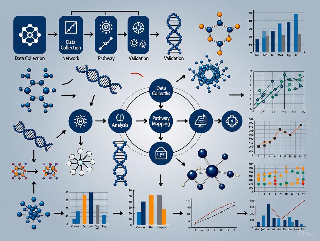
Systems Biology Approaches to Biomarker Discovery

Integrated Computational-Experimental Workflows

Systems biology employs data-driven, knowledge-based approaches that effectively integrate high-throughput experimental data with existing biological knowledge to identify robust biomarkers [2]. This methodology recognizes that meaningful biomarkers often reflect perturbations in interconnected biological networks rather than isolated molecular changes. A representative workflow for glioblastoma multiforme (GBM) biomarker discovery exemplifies this approach, beginning with dataset retrieval from public repositories like the Gene Expression Omnibus (GEO), followed by identification of differentially expressed genes (DEGs) using statistical methods including p-values and false discovery rates [3].

The systems biology pipeline proceeds with survival and expression analysis to establish clinical relevance, construction of protein-protein interaction (PPI) networks to identify hub genes, and functional enrichment analysis to elucidate biological pathways [3]. The process culminates in molecular docking and dynamic simulation of potential therapeutic compounds, creating a comprehensive framework that connects biomarker identification to therapeutic development [3]. This integrated approach successfully identified matrix metallopeptidase 9 (MMP9) as a key hub gene in GBM, with molecular docking studies revealing high binding affinities for therapeutic compounds including temozolomide (-8.7 kcal/mol) and marimastat (-7.7 kcal/mol) [3].

Systems Biology Biomarker Discovery Workflow

Multi-Omics Integration and Network Analysis

The integration of multi-omics data represents a cornerstone of systems biology approaches to biomarker discovery [5]. By simultaneously analyzing genomics, transcriptomics, proteomics, and metabolomics data, researchers can develop comprehensive molecular maps of diseases and identify complex biomarker signatures that would be undetectable through single-omics approaches [4]. This strategy captures dynamic molecular interactions between biological layers, revealing pathogenic mechanisms that remain invisible when examining individual molecular classes in isolation [4].

Network-based analysis of molecular interactions has emerged as a powerful method for identifying robust biomarkers that reflect the underlying biology of disease [2]. By constructing and analyzing protein-protein interaction networks, gene regulatory networks, and signaling pathways, researchers can identify hub genes and proteins that occupy central positions in disease-relevant networks [3]. In the GBM study, network analysis revealed MMP9 as the highest-degree hub gene, followed by periostin (POSTN) and Hes family BHLH transcription factor 5 (HES5), highlighting their potential importance in disease pathogenesis [3]. This network-based approach to biomarker discovery captures changes in downstream effectors and frequently yields more powerful predictors compared to individual molecules [2].

Application Notes: Protocol for Longitudinal Biomarker Discovery

Study Design and Cohort Establishment

The International Network of Special Immunization Services (INSIS) has established a comprehensive protocol for longitudinal biomarker discovery focused on vaccine safety [6] [7]. This meta-cohort study employs systems biology to identify biomarkers of rare adverse events following immunization (AEFIs), implementing harmonized case definitions and standardized protocols for collecting data and samples related to conditions such as myocarditis, pericarditis, and Vaccine-Induced Immune Thrombocytopenia and Thrombosis (VITT) after COVID-19 vaccinations [7]. The network ensures accurate and standardized data collection through rigorous data management and quality assurance processes, creating a robust foundation for biomarker identification [6].

The INSIS protocol integrates clinical data with multi-omics technologies including transcriptomics, proteomics, and metabolomics through a global consortium of clinical networks [7]. This integrated approach facilitates the uncovering of molecular mechanisms behind AEFIs by leveraging expertise from immunology, pharmacogenomics, and systems biology teams [6]. The study design enhances risk-benefit assessments of vaccines across populations, identifies actionable biomarkers to inform discovery and development of safer vaccines, and supports personalized vaccination strategies [7].

Data Integration and Analytical Framework

The INSIS protocol implements a structured data integration and analytical framework that combines clinical phenotyping with comprehensive molecular profiling [7]. The approach employs rigorous statistical methods for identifying differentially expressed genes and proteins, followed by network analysis to identify central players in vaccine adverse event pathways [6]. This methodology enables the discovery of biomarker signatures that reflect the complex biological processes underlying rare adverse events, moving beyond single-marker approaches to capture the systems-level interactions that characterize immunological responses [7].

The analytical framework incorporates longitudinal sampling strategies that capture dynamic changes in molecular profiles over time, providing valuable information about the temporal progression of vaccine responses and adverse events [6]. This temporal dimension is particularly important for understanding the evolution of biological processes and identifying biomarkers that may appear at specific timepoints following vaccination [7]. The integration of longitudinal molecular data with detailed clinical phenotyping creates a powerful resource for identifying biomarkers with predictive value for vaccine safety assessment [6].

The Scientist's Toolkit: Research Reagent Solutions

Table: Essential Research Reagents and Platforms for Biomarker Discovery

Reagent/Platform	Function	Application Context
Affymetrix Microarray Platforms	Genome-wide expression profiling	Identification of differentially expressed genes [3]
Liquid Chromatography-Mass Spectrometry (LC-MS)	Proteomic and metabolomic profiling	Comprehensive molecular signature identification [4] [7]
OpenArray miRNA Panels	High-throughput miRNA quantification	Circulating miRNA biomarker discovery [2]
Proximity Extension Assays (PEA)	High-sensitivity protein detection	Multiplexed protein biomarker validation [7]
Single-cell RNA Sequencing	Resolution of cellular heterogeneity	Identification of rare cell populations [5]
MirVana PARIS miRNA Isolation Kit	RNA extraction from biofluids	Preparation of circulating miRNA samples [2]
Hsd17B13-IN-40	Hsd17B13-IN-40|HSD17B13 Inhibitor
Fluplatin	Fluplatin, MF:C48H56F2N4O8Pt, MW:1050.1 g/mol	Chemical Reagent

Analytical and Validation Methodologies

Computational Analysis Pipelines

Bioinformatics pipelines for biomarker discovery incorporate multiple analytical steps to ensure robust identification of clinically relevant biomarkers. The GBM biomarker discovery protocol begins with data preprocessing and normalization of gene expression datasets, followed by identification of differentially expressed genes (DEGs) using statistical methods including p-values and false discovery rates (FDR) [3]. This initial analysis identified 132 significant genes in GBM, with 13 showing upregulation and 29 showing unique downregulation [3].

Advanced computational methods include principal component analysis (PCA) to organize data with related properties, construction of protein-protein interaction (PPI) networks specifically focused on DEGs, and identification of hub genes within these networks using connectivity measures [3]. Functional enrichment analysis using KEGG pathways and Gene Ontology terms elucidates the biological processes, cellular components, and molecular functions associated with identified biomarker candidates [3]. These computational approaches are complemented by survival analysis to establish clinical relevance and molecular docking studies to explore therapeutic targeting of identified biomarkers [3].

Data Integration and Analysis Pipeline

Validation and Clinical Translation

Analytical validation establishes that biomarker measurements work consistently and accurately, assessing performance characteristics including sensitivity, specificity, accuracy, precision, and robustness [1]. This process requires standardization to ensure biomarkers produce identical results across different laboratories, platforms, and technicians [1]. Regulatory agencies demand extensive analytical validation data before approving biomarker-guided therapies, making this a critical step in the biomarker development pipeline [1].

Clinical validation represents the ultimate test of biomarker utility, demonstrating that biomarkers actually improve patient outcomes or clinical decision-making in real-world settings [1]. Successful clinical validation typically requires large-scale studies with appropriate patient populations and meaningful clinical endpoints, establishing clinical utility through improved patient outcomes, reduced healthcare costs, or enhanced treatment selection compared to existing approaches [1]. The transition from analytical to clinical validation represents a significant challenge in biomarker development, with many promising candidates failing to demonstrate sufficient clinical utility for widespread adoption [4].

Emerging Trends and Future Directions

The field of biomarker discovery is rapidly evolving, with several emerging trends shaping future research directions. Artificial intelligence and machine learning are playing increasingly important roles in biomarker analysis, enabling sophisticated predictive models that forecast disease progression and treatment responses based on biomarker profiles [5]. AI-driven algorithms facilitate automated interpretation of complex datasets, significantly reducing the time required for biomarker discovery and validation [4] [5]. By 2025, AI integration is expected to enable more personalized treatment plans through analysis of individual patient data alongside biomarker information [5].

Liquid biopsy technologies are poised to become standard tools in clinical practice, with advances in circulating tumor DNA (ctDNA) analysis and exosome profiling increasing the sensitivity and specificity of these non-invasive approaches [5]. Liquid biopsies facilitate real-time monitoring of disease progression and treatment responses, allowing for timely adjustments in therapeutic strategies [5]. While initially focused on oncology applications, liquid biopsies are expanding into other medical areas including infectious diseases and autoimmune disorders [5]. These technological advances, combined with evolving regulatory frameworks and increased emphasis on patient-centric approaches, are driving significant advancements in biomarker development and implementation [5].

The Limitation of Single-Target Biomarkers and the Rise of Multi-Omics Panels

The field of biomarker discovery is undergoing a fundamental transformation, moving from a traditional reductionist approach that focuses on single molecules to a holistic, systems-based approach that integrates multiple layers of biological information. Biomarkers, defined as objectively measurable indicators of biological processes, pathogenic processes, or pharmacological responses, have long been cornerstone tools in disease diagnosis, prognosis, and treatment selection [8] [4]. However, the complexity and heterogeneity of human diseases, particularly cancer and neurodegenerative disorders, have exposed critical limitations in single-target biomarkers, driving the emergence of multi-omics panels that provide a more comprehensive view of disease mechanisms [9] [10].

Traditional single-target biomarkers often fail to capture the multifaceted nature of complex diseases. The over-reliance on hypothesis-driven, reductionist approaches has limited the translation of fundamental research into new clinical applications due to their limited ability to unravel the multivariate and combinatorial characteristics of cellular networks implicated in multi-factorial diseases [2]. In contrast, multi-omics strategies integrate various molecular layers—including genomics, transcriptomics, proteomics, metabolomics, and epigenomics—to develop composite signatures that more accurately reflect disease complexity [9] [11]. This paradigm shift aligns with the core principles of systems biology, which views biological systems as integrated networks and focuses on understanding disease-perturbed molecular networks as the fundamental causes of pathology [10] [12].

Critical Limitations of Single-Target Biomarkers

Biological and Technical Challenges

Single-target biomarkers face substantial challenges that limit their clinical utility across diverse patient populations. These limitations stem from both biological complexity and technical constraints, including:

• Disease Heterogeneity: Complex diseases like cancer and neurodegenerative disorders involve multiple molecular pathways and cell types. Single biomarkers cannot adequately capture this heterogeneity, leading to misclassification and incomplete pathological characterization [10] [2]. For example, the HER2 biomarker for breast cancer, while groundbreaking, shows ongoing debate about optimal assay methodology and efficacy in patients with varying expression levels [13].

• Limited Sensitivity and Specificity: Individual biomarkers often lack sufficient predictive power for reliable clinical decision-making. This limitation is particularly evident in early disease detection, where single markers may not reach the required accuracy thresholds for population screening [4].

• Susceptibility to Analytical Variability: Measurements of single biomarkers can be affected by numerous preanalytical and analytical factors, including sample collection methods, storage conditions, and assay technical variability [8] [13].

• Inadequate Representation of System Dynamics: Biological systems are dynamic and adaptive. Single-timepoint measurements of individual biomarkers cannot capture the temporal evolution of disease processes or the complex interactions between different biological pathways [10] [4].

Clinical Implementation Challenges

The transition from biomarker discovery to clinical implementation reveals additional limitations of single-target approaches:

• Limited Prognostic and Predictive Value: While some single biomarkers have proven useful for diagnosis, they often provide incomplete information for prognosis or treatment selection. The distinction between prognostic markers (indicating disease outcome regardless of treatment) and predictive markers (indicating response to specific therapies) is crucial clinically, yet few single biomarkers fulfill both roles effectively [13] [14].

• Insufficient Guidance for Personalized Therapy: The vision of precision medicine requires biomarkers that can guide therapy selection for individual patients. Single biomarkers typically address only one aspect of a drug's mechanism of action, failing to account for the complex network perturbations that influence treatment response [9] [10].

• High False Discovery Rates: In large-scale omics studies, focusing on individual molecules without considering their biological context increases the risk of identifying false associations that fail validation in independent cohorts [2].

Table 1: Comparative Analysis of Single-Target vs. Multi-Omics Biomarkers

Characteristic	Single-Target Biomarkers	Multi-Omics Panels
Biological Coverage	Limited to one molecular layer	Comprehensive across multiple biological layers
Handling of Heterogeneity	Poor capture of disease diversity	Stratification based on integrated patterns
Predictive Power	Often modest (AUC 0.6-0.8)	Enhanced through complementary signals (AUC >0.9 possible)
Technical Variability	Highly susceptible to preanalytical factors	Robust through consensus across platforms
Clinical Utility	Limited to specific contexts	Broad application across diagnosis, prognosis, and treatment
Development Timeline	Typically shorter discovery phase	Extended integration and validation required

The Multi-Omics Approach: Theoretical Foundations and Technological Advances

Systems Biology as the Conceptual Framework

The rise of multi-omics panels is grounded in systems biology, which approaches biology as an information science and studies biological systems as a whole, including their interactions with the environment [10] [12]. This approach recognizes that disease arises from perturbations in molecular networks rather than alterations in single molecules. Systems biology employs five key features that enable effective multi-omics biomarker discovery:

• Global molecular measurements across multiple biological layers (genome, transcriptome, proteome, metabolome)
• Information integration across these different levels to understand system-environment interactions
• Analysis of dynamic changes in biological systems as they adapt and respond to perturbations
• Computational modeling through integration of global and dynamic data
• Iterative prediction and validation to refine models and biomarkers [10]

This framework enables the identification of "disease-perturbed networks" whose molecular fingerprints can be detected in patient samples and used for disease detection and stratification [10]. The core premise is that molecular signatures resulting from network perturbations provide more robust and clinically informative biomarkers than single molecules.

Technological Enablers of Multi-Omics Research

Several technological advances have made multi-omics biomarker discovery feasible:

• High-Throughput Sequencing Technologies: Next-generation sequencing platforms have dramatically reduced the cost and increased the speed of genomic, transcriptomic, and epigenomic profiling [9].

• Advanced Mass Spectrometry: Innovations in liquid chromatography-mass spectrometry (LC-MS) and other proteomic/metabolomic technologies enable comprehensive protein and metabolite profiling [9] [4].

• Single-Cell and Spatial Omics: Emerging technologies allow molecular profiling at single-cell resolution and within spatial context, capturing cellular heterogeneity and tissue organization [9] [11].

• Computational and AI Tools: Machine learning algorithms, particularly deep learning networks, can integrate high-dimensional multi-omics data to identify complex patterns beyond human perception [9] [14].

The following diagram illustrates the conceptual framework of multi-omics integration in systems biology:

Multi-Omics Integration Strategies and Methodologies

Data Types and Their Clinical Applications

Multi-omics encompasses large-scale analyses of multiple molecular layers, each providing unique insights into biological processes and disease mechanisms. The major omics technologies and their applications in biomarker discovery include:

• Genomics: Investigates DNA-level alterations including copy number variations, genetic mutations, and single nucleotide polymorphisms using whole exome sequencing (WES) and whole genome sequencing (WGS). Clinical applications include tumor mutational burden (TMB) as a predictive biomarker for immunotherapy response [9].

• Transcriptomics: Explores RNA expression patterns using microarrays and RNA sequencing, encompassing mRNAs, long noncoding RNAs, and microRNAs. Clinically validated applications include the Oncotype DX (21-gene) and MammaPrint (70-gene) assays for breast cancer prognosis [9].

• Proteomics: Investigates protein abundance, modifications, and interactions using mass spectrometry and protein arrays. Proteomic profiling can identify functional subtypes and druggable vulnerabilities missed by genomics alone [9].

• Epigenomics: Examines DNA and histone modifications including DNA methylation and histone acetylation using whole genome bisulfite sequencing and ChIP-seq. MGMT promoter methylation in glioblastoma represents a classic clinical biomarker predicting temozolomide response [9].

• Metabolomics: Analyzes cellular metabolites including small molecules, lipids, and carbohydrates using LC-MS and GC-MS. The oncometabolite 2-hydroxyglutarate (2-HG) serves as both diagnostic and mechanistic biomarker in IDH1/2-mutant gliomas [9].

Table 2: Multi-Omics Data Types and Their Biomarker Applications

Omics Layer	Measured Molecules	Primary Technologies	Example Clinical Biomarkers
Genomics	DNA sequences, mutations, CNVs	WGS, WES, SNP arrays	Tumor mutational burden, BRCA1/2 mutations
Transcriptomics	mRNA, lncRNA, miRNA	RNA-seq, Microarrays	Oncotype DX, MammaPrint
Proteomics	Proteins, PTMs	LC-MS/MS, RPPA	HER2 overexpression, PSA
Epigenomics	DNA methylation, histone modifications	WGBS, ChIP-seq	MGMT promoter methylation
Metabolomics	Metabolites, lipids	LC-MS, GC-MS, NMR	2-hydroxyglutarate in IDH-mutant glioma

Computational Integration Methods

Integrating multi-omics data presents significant computational challenges due to high dimensionality, heterogeneity, and noise. Several strategies have been developed to address these challenges:

• Horizontal Integration: Combines the same type of omics data across multiple samples or studies to increase statistical power and identify consistent patterns. This approach requires careful batch effect correction and normalization [9].

• Vertical Integration: Simultaneously analyzes different types of omics data from the same samples to build comprehensive molecular models. Network-based approaches are particularly powerful for vertical integration, revealing key molecular interactions and biomarkers [9] [11].

• AI-Powered Integration: Machine learning and deep learning algorithms can identify complex, non-linear relationships across omics layers. Random forests, support vector machines, and neural networks have demonstrated particular utility for multi-omics biomarker discovery [14].

The following workflow diagram illustrates a typical multi-omics integration pipeline for biomarker discovery:

Application Notes: Protocol for Multi-Omics Biomarker Discovery

Case Study: Integrated Transcriptomic and DNA Methylation Analysis in Periodontitis

The following protocol outlines a robust methodology for multi-omics biomarker discovery, adapted from a study integrating transcriptomic and DNA methylation profiles to identify immune-associated biomarkers in periodontitis [15]. This approach can be adapted to various disease contexts with appropriate modifications.

Sample Preparation and Data Acquisition

Materials and Reagents:

• Illumina Human Methylation EPIC Array or equivalent methylation bead chip
• RNA extraction kit (e.g., MirVana PARIS miRNA isolation kit)
• RNA quality control tools (e.g., Implen Nanophotometer)
• Real-time RT-qPCR equipment and reagents
• Appropriate microarray or sequencing platforms for transcriptomic profiling

Procedure:

• Sample Collection: Obtain diseased and healthy control tissues matched for relevant clinical parameters. For the periodontitis study, 12 patients and 12 healthy controls were used [15].
• DNA Methylation Profiling:
  • Process samples using the Illumina Human Methylation EPIC Array covering >810,000 methylation sites
  • Remove probes with null values, those located on sex chromosomes, and probes mapping to multiple genes or containing SNPs
  • Normalize raw data using the minfi R package
  • Identify differentially methylated probes with p-value < 0.05 and absolute detabeta (|Δβ|) > 0.1
• Transcriptomic Profiling:
  • Extract total RNA following manufacturer protocols
  • Perform quality control assessment for haemolysis by examining free haemoglobin and miRNA levels
  • Conduct global profiling using appropriate platforms (microarray or RNA-seq)
  • Identify differentially expressed genes using the limma R package with adjusted p-value < 0.05 and absolute log2 fold change ≥ 0.263

Immune Microenvironment Characterization

Procedure:

• Immune Cell Abundance Estimation:
  • Use the xcell R package to estimate abundance of 64 immune cell types
  • Compare immune cell profiles between disease and control groups to identify significantly altered cell populations
• Correlation Analysis:
  • Perform Pearson correlation analysis between DNA methylation levels and gene expression
  • Consider only correlations with absolute Pearson coefficient > 0.4 and p-value < 0.05 statistically significant

Integrative Bioinformatics Analysis

Computational Tools:

• R packages: WGCNA, randomForest, e1071 (SVM implementation)
• Metascape webserver for functional enrichment analysis

Procedure:

• Weighted Gene Co-expression Network Analysis (WGCNA):
  • Construct co-expression networks using the WGCNA R package
  • Identify gene modules correlated with altered immune cell populations
  • Select hub genes within significant modules for further analysis
• Machine Learning-Based Biomarker Identification:
  • Build prediction models using random forest method via the randomForest R package
  • Identify optimal gene combinations with high discriminatory power
  • Apply support vector machine (SVM) algorithm using the e1071 package to refine diagnostic models
  • Validate key genes across independent datasets (e.g., 247 and 310 samples in the periodontitis study)
• Functional Enrichment Analysis:
  • Perform enrichment analysis of differentially expressed genes and differentially methylated genes using Metascape
  • Analyze KEGG pathways and Hallmark gene sets with false discovery rate < 0.05

Case Study: Network-Based microRNA Biomarker Discovery in Colorectal Cancer

This protocol outlines a data-driven, knowledge-based approach for identifying circulating microRNA biomarkers of colorectal cancer prognosis, adapted from a study that integrated miRNA expression with miRNA-mediated regulatory networks [2].

Sample Processing and miRNA Profiling

Materials and Reagents:

• Blood collection tubes (e.g., K3EDTA tubes)
• Centrifuge capable of 2500 × g
• MirVana PARIS miRNA isolation kit
• OpenArray platform or equivalent high-throughput miRNA profiling system
• ViiA 7 instrument or equivalent real-time PCR system

Procedure:

• Blood Collection and Plasma Preparation:
  • Collect blood via venepuncture in K3EDTA tubes
  • Invert tubes 10 times immediately after collection
  • Centrifuge at 2500 × g for 20 minutes at room temperature within 30 minutes of collection
  • Store plasma at -80°C until RNA isolation
• RNA Isolation and Quality Control:
  • Isolate total RNA from plasma using the MirVana PARIS kit with modified protocol
  • Assess haemolysis by examining free haemoglobin and miR-16 levels
  • Exclude haemolysed samples from further analysis
• miRNA Profiling:
  • Conduct global miRNA profiling using the OpenArray platform per manufacturer's instructions
  • Use entire RT reaction for pre-amplification on a ViiA 7 instrument
  • Combine resultant cDNA with OpenArray real-time PCR Master Mix
  • Load onto OpenArray miRNA panel plates using the AccuFill autoloader
  • Run according to default protocol for reaction conditions

Data Preprocessing and Normalization

Computational Tools:

• MATLAB Bioinformatics Toolbox and Statistics Toolbox
• R statistical environment with DMwR package

Procedure:

• Quality Assessment and Normalization:
  • Preprocess miRNA cycle quantification (Cq) values from RT-qPCR assays
  • Perform quantile normalization to adjust for technical variability
  • Exclude miRNAs missing in >50% of samples
  • Impute missing data using the nearest-neighbor method (KNNimpute)
• Class Definition and Balancing:
  • Dichotomize patients into long vs. short survival using clinical endpoints (e.g., 2-year cut-off)
  • Address unbalanced class distribution using Synthetic Minority Oversampling Technique (SMOTE) via the R DMwR package during model selection only
• Differential Expression Analysis:
  • Perform non-parametric tests (Kolmogorov-Smirnov and Wilcoxon) due to non-normal data distribution
  • Test the null hypothesis that miRNA Cq values in short vs. long survival patients are from the same continuous distribution

Network-Based Biomarker Identification

Procedure:

• Multi-Objective Optimization Framework:
  • Formulate biomarker identification as an optimization problem
  • Integrate miRNA expression data with knowledge from miRNA-mediated regulatory networks
  • Identify robust plasma miRNA signatures with both predictive power and functional relevance
• Validation:
  • Confirm altered expression of identified miRNAs in independent public datasets
  • Validate the prognostic signature comprising 11 circulating miRNAs for colorectal cancer

The Scientist's Toolkit: Essential Research Reagent Solutions

Successful multi-omics biomarker discovery requires carefully selected reagents and platforms optimized for integrative analyses. The following table details essential research tools and their applications in multi-omics studies:

Table 3: Essential Research Reagent Solutions for Multi-Omics Biomarker Discovery

Reagent/Platform	Manufacturer/Provider	Primary Application	Key Features
Illumina Methylation EPIC Array	Illumina	DNA methylation profiling	Covers >810,000 methylation sites, comprehensive genome coverage
MirVana PARIS miRNA Isolation Kit	Ambion/Applied Biosystems	miRNA extraction from plasma	Optimized for small RNA recovery, suitable for liquid biopsies
OpenArray miRNA Panels	Applied Biosystems	High-throughput miRNA profiling	Preconfigured panels, suitable for biomarker validation studies
minfi R Package	Bioconductor	Methylation data normalization	Specialized tools for processing Illumina methylation array data
WGCNA R Package	CRAN	Co-expression network analysis	Identifies modules of highly correlated genes, links to clinical traits
xCell R Package	CRAN	Immune cell type enrichment	Estimates abundance of 64 immune cell types from gene expression data
LC-MS/MS Systems	Multiple vendors	Proteomic and metabolomic profiling	High sensitivity and specificity for protein/metabolite identification
Random Forest Algorithm	Multiple implementations	Machine learning classification	Handles high-dimensional data, provides variable importance measures
Hsd17B13-IN-59	Hsd17B13-IN-59, MF:C24H17Cl2N5O3, MW:494.3 g/mol	Chemical Reagent	Bench Chemicals
Anticancer agent 177	Anticancer agent 177, MF:C28H36Cl2N4O2, MW:531.5 g/mol	Chemical Reagent	Bench Chemicals

The transition from single-target biomarkers to multi-omics panels represents a fundamental evolution in biomarker science, driven by the recognition that complex diseases require comprehensive, systems-level approaches. Multi-omics integration provides unprecedented opportunities to capture disease heterogeneity, identify robust diagnostic and prognostic signatures, and guide personalized treatment decisions [9] [11].

Despite these advances, significant challenges remain in the widespread implementation of multi-omics biomarkers. Data heterogeneity, analytical standardization, and the complexity of clinical validation present substantial hurdles [4] [13]. Future developments will likely focus on several key areas:

• Standardization of Analytical Frameworks: Establishment of standardized protocols for multi-omics data generation, processing, and integration to improve reproducibility across studies [9] [4].

• Advanced Computational Methods: Further development of AI and machine learning approaches, particularly explainable AI that provides transparent, interpretable results for clinical decision-making [14].

• Single-Cell and Spatial Multi-Omics: Integration of single-cell sequencing with spatial transcriptomics and proteomics to capture cellular heterogeneity and tissue context [9] [11].

• Longitudinal Monitoring: Implementation of serial multi-omics profiling to track disease progression and treatment response over time [4].

• Federated Learning Approaches: Development of privacy-preserving analytical methods that enable multi-institutional collaboration without sharing sensitive patient data [14].

The continued evolution of multi-omics biomarker discovery holds tremendous promise for advancing precision medicine, enabling earlier disease detection, more accurate prognosis, and personalized therapeutic interventions tailored to individual molecular profiles.

Systems biology represents a paradigm shift in biomedical research, moving from a reductionist study of individual molecules to a holistic analysis of complex biological systems as a whole. By integrating large-scale molecular data with computational modeling, this approach recognizes that biological information is captured, transmitted, and integrated by networks of molecular components [10]. For biomarker discovery, this translates to identifying disease-perturbed molecular networks rather than single molecules, providing more robust and clinically meaningful signatures [10] [2]. The core principles outlined in this document—network analysis, pathway integration, and multi-omics data synthesis—are revolutionizing how researchers identify biomarkers for personalized medicine, drug development, and therapeutic optimization.

Table 1: Core Systems Biology Principles in Biomarker Discovery

Principle	Description	Impact on Biomarker Discovery
Network Analysis	Studies biological systems as interconnected networks rather than isolated components	Identifies robust biomarkers that capture system-level perturbations beyond individual gene/protein expression [2]
Pathway Integration	Maps molecular changes onto predefined biological pathways and processes	Provides functional context, revealing mechanisms behind biomarker candidates and improving interpretability [16] [17]
Multi-Omics Data Synthesis	Integrates data from genomics, transcriptomics, proteomics, and metabolomics	Generates comprehensive biomarker signatures that reflect disease complexity [5] [7]
Dynamic Modeling	Analyzes how biological systems change over time and respond to perturbations	Enables identification of early-warning biomarkers before clinical symptom manifestation [10]

Traditional approaches to biomarker discovery have primarily relied on differential expression analysis of individual molecules. While valuable, this reductionist method often fails to capture the multivariate and combinatorial characteristics of cellular networks implicated in multi-factorial diseases [2]. Systems biology addresses this limitation by providing a framework to understand how interactions between biological components give rise to emergent properties and complex phenotypes.

The fundamental shift involves viewing biology as an information science, where disease states emerge from perturbations in biological networks [10]. This perspective has proven particularly powerful for deciphering complex pathologies including neurodegenerative diseases, cancer, and adverse drug reactions [10] [7]. The five key features of contemporary systems biology include: (1) quantification of global biological information, (2) integration across different biological levels (DNA, RNA, protein), (3) study of dynamical system changes, (4) computational modeling of biological systems, and (5) iterative model testing and refinement [10].

For biomarker research, this approach enables the identification of "molecular fingerprints" resulting from disease-perturbed networks, which can detect and stratify various pathological conditions with greater accuracy than single-parameter biomarkers [10]. These fingerprints can comprise proteins, DNA, RNA, microRNAs, metabolites, and their post-translational modifications, providing multi-parameter analyses that reflect the true complexity of disease states [10].

Experimental Protocols

Protocol 1: Network-Based Biomarker Discovery Using PageRank Algorithm

Purpose: To identify functionally relevant biomarkers by integrating protein-protein interaction networks with gene expression data and biological pathways for predicting response to immune checkpoint inhibitors (ICIs) [16].

Background: Predicting ICI response remains challenging in cancer immunotherapy. Conventional methods relying on differential gene expression or predefined immune signatures often fail to capture complex regulatory mechanisms. Network-based models like PathNetDRP address this by quantitatively assessing how individual genes contribute within pathways, improving both specificity and interpretability of biomarkers [16].

Table 2: Reagents and Equipment for Network-Based Biomarker Discovery

Item	Specification	Purpose
Transcriptomic Data	RNA-seq from ICI-treated patient cohorts	Input for differential expression analysis and pathway activity mapping [16]
Protein-Protein Interaction Network	STRING database or similar	Framework for network propagation and identifying functionally related genes [16]
Pathway Databases	Reactome, KEGG, GO	Biological context for interpreting identified biomarker candidates [16] [17]
Computational Environment	R/Python with igraph, numpy, pandas	Implementation of PageRank algorithm and statistical analyses [16]

Procedure:

• ICI-Related Gene Selection via PageRank:
  • Initialize gene scores using known ICI target genes
  • Apply PageRank algorithm to PPI network to propagate influence across the network
  • Iteratively update gene scores using the formula: PR(gi;t) = (1-d)/N + d * Σ PR(gj; t-1)/L(gj) where gi is the gene of interest, d is the damping factor, N is the total number of genes, and L(gj) is the number of neighbors of gene gj [16]
  • Select top-ranked genes as candidate biomarkers

• Identification of ICI-Related Biological Pathways:

  • Map candidate genes to biological pathways using hypergeometric testing
  • Apply multiple testing correction (e.g., Benjamini-Hochberg) to control false discovery rate
  • Select pathways with significant enrichment of candidate genes (FDR < 0.05)

• Calculation of PathNetGene Scores:

  • Construct pathway-specific subnetworks from significant pathways
  • Apply PageRank to each subnetwork to quantify gene importance within pathways
  • Calculate final PathNetGene scores by combining network topology and expression data

• Biomarker Validation:

  • Validate predictive performance using leave-one-out cross-validation and independent validation cohorts
  • Compare against state-of-the-art methods (e.g., TIDE, IMPRES, DeepGeneX) using area under ROC curve as primary metric [16]

Expected Outcomes: PathNetDRP has demonstrated strong predictive performance with AUC increasing from 0.780 to 0.940 in cross-validation compared to conventional methods. The approach identifies novel biomarker candidates while providing insights into key immune-related pathways [16].

Protocol 2: Pathway-Centric Analysis Using Biologically Informed Neural Networks (BINNs)

Purpose: To enhance proteomic biomarker discovery and pathway analysis by integrating a priori knowledge of protein-pathway relationships into interpretable neural networks [17].

Background: Deep learning models offer powerful predictive capabilities but typically suffer from lack of interpretability. BINNs address this limitation by constructing sparse neural networks where connections reflect established biological relationships, enabling simultaneous biomarker identification and pathway analysis [17].

Table 3: Reagents and Equipment for BINN Analysis

Item	Specification	Purpose
Proteomics Data	Mass spectrometry or Olink platform data	Input for classifying clinical subphenotypes [17]
Pathway Database	Reactome database	Source of biological relationships for network construction [17]
Software Package	BINN Python package (GitHub)	Implementation of biologically informed neural networks [17]
Interpretation Tools	SHAP (Shapley Additive Explanations)	Model interpretation and feature importance calculation [17]

Procedure:

• Data Preparation:
  • Quantify proteins using proteotypic peptides to ensure unique protein group membership
  • Stratify patients into clinical subphenotypes (e.g., septic AKI subphenotypes 1 and 2, or COVID-19 severity according to WHO scale)
  • Perform standard preprocessing including normalization and quality control

• BINN Construction:

  • Extract relevant biological entities from Reactome database
  • Subset and layerize the Reactome graph to fit a sequential neural network structure
  • Translate the layered graph to a sparse neural network architecture with nodes annotated as proteins, pathways, or biological processes
  • Construct input layer with proteins, hidden layers with pathways, and output layer with clinical subphenotypes

• Model Training and Validation:

  • Train BINN to classify subphenotypes using proteome as input
  • Employ k-fold cross-validation (k=3) for performance evaluation
  • Benchmark against other machine learning methods (SVM, random forest, XGBoost) using AUC metrics

• Model Interpretation:

  • Apply SHAP to calculate feature importance for proteins and pathways
  • Identify important proteins based on highest mean absolute SHAP values
  • Extract significant pathways by aggregating SHAP values at pathway nodes
  • Validate biological relevance through literature review and functional annotation

Expected Outcomes: BINNs have achieved ROC-AUC of 0.99 ± 0.00 for septic AKI subphenotypes and 0.95 ± 0.01 for COVID-19 severity, outperforming conventional machine learning methods. The approach identifies panels of potential protein biomarkers and provides molecular explanations for clinical subphenotypes [17].

Visualization of Systems Biology Workflows

Pathway-Centric Biomarker Discovery Workflow

Network Propagation in PathNetDRP

The Scientist's Toolkit: Research Reagent Solutions

Table 4: Essential Research Reagents and Platforms for Systems Biology Biomarker Discovery

Category	Specific Products/Platforms	Function in Workflow
Multi-omics Profiling	Next-generation sequencing (NGS), Mass spectrometry, Olink platform	Generation of comprehensive molecular data from genomics, transcriptomics, and proteomics [5] [17]
Pathway Databases	Reactome, KEGG, Gene Ontology, STRING	Source of curated biological knowledge for network construction and functional annotation [16] [17]
Computational Tools	BINN Python package, PathNetDRP, R/Bioconductor	Implementation of specialized algorithms for network analysis and biomarker prioritization [16] [17]
Liquid Biopsy Technologies	Circulating tumor DNA (ctDNA) analysis, Exosome profiling	Non-invasive sample collection for real-time disease monitoring and treatment response assessment [5]
AI and Machine Learning	SHAP, PyTorch, scikit-learn	Model interpretation, feature importance calculation, and predictive analytics [5] [17]
Retagliptin hydrochloride	Retagliptin hydrochloride, CAS:1174038-86-8, MF:C19H19ClF6N4O3, MW:500.8 g/mol	Chemical Reagent
Hsd17B13-IN-61	Hsd17B13-IN-61|Potent HSD17B13 Inhibitor for NAFLD/NASH Research	Hsd17B13-IN-61 is a potent inhibitor of the HSD17B13 enzyme. It is For Research Use Only and is a valuable tool for investigating chronic liver diseases like NAFLD and NASH.

Future Perspectives

The field of systems biology-driven biomarker discovery continues to evolve rapidly. Several emerging trends are poised to shape future research. By 2025, enhanced integration of artificial intelligence and machine learning will enable more sophisticated predictive models that can forecast disease progression and treatment responses based on comprehensive biomarker profiles [5]. Multi-omics approaches are expected to gain further momentum, with researchers increasingly leveraging combined data from genomics, proteomics, metabolomics, and transcriptomics to achieve a holistic understanding of disease mechanisms [5].

Liquid biopsy technologies are advancing toward becoming standard tools in clinical practice, with improvements in sensitivity and specificity for circulating tumor DNA analysis and exosome profiling [5]. These technologies will facilitate real-time monitoring of disease progression and treatment responses, enabling timely adjustments in therapeutic strategies. Single-cell analysis technologies are also becoming more sophisticated and widely adopted, providing deeper insights into tumor microenvironments and enabling identification of rare cell populations that may drive disease progression or therapy resistance [5].

From a regulatory perspective, frameworks are adapting to ensure new biomarkers meet necessary standards for clinical utility. Streamlined approval processes, standardization initiatives, and emphasis on real-world evidence will be key developments by 2025 [5]. Finally, the field is increasingly focusing on patient-centric approaches, with biomarker analysis playing a key role in enhancing patient engagement and outcomes through informed consent practices, incorporation of patient-reported outcomes, and engagement of diverse populations [5].

The integration of multiple biological data layers—genomics, transcriptomics, proteomics, metabolomics, and microbiomics—represents a foundational paradigm shift in biomarker discovery within systems biology. This multi-omics approach enables researchers to move beyond single-layer analysis to a holistic understanding of the complex molecular networks driving health and disease. By simultaneously interrogating multiple molecular levels, systems biology approaches can identify robust biomarker signatures that account for biological complexity, heterogeneity, and dynamic regulation. The convergence of these data layers is particularly powerful in precision oncology, neurodegenerative disease research, and complex chronic conditions where single biomarkers often lack sufficient sensitivity or specificity.

High-dimensional molecular studies in biofluids have demonstrated particular promise for scalable biomarker discovery, though challenges in assembling large, diverse datasets have historically hindered progress [18]. Recent technological advances in high-throughput sequencing, mass spectrometry, and computational biology are now overcoming these barriers, enabling the comprehensive profiling required for clinically actionable biomarker identification. The strategic integration of these omics layers facilitates the discovery of biomarkers that can improve early detection, prognosis, staging, and subtyping of complex diseases [18] [9].

Omics Technologies and Their Applications in Biomarker Discovery

Genomics

Genomics investigates alterations at the DNA level, providing a fundamental blueprint of an organism's genetic makeup and its associations with disease states. Advanced sequencing technologies, including whole exome sequencing (WES) and whole genome sequencing (WGS), enable the identification of copy number variations (CNVs), genetic mutations, and single nucleotide polymorphisms (SNPs) [9]. Genome-wide association studies (GWAS) have been instrumental in identifying cancer-associated genetic variations, providing a foundational resource for potential cancer biomarkers [9].

In clinical practice, genomic biomarkers have become essential tools for guiding targeted therapies. For example, the tumor mutational burden (TMB), validated in the KEYNOTE-158 trial, has been approved by the FDA as a predictive biomarker for pembrolizumab treatment across solid tumors [9]. Similarly, identifying HER2 gene amplification in breast cancer guides targeted therapy choices, while detecting EGFR mutations in lung cancer patients allows for tailored treatments with tyrosine kinase inhibitors [19]. The adoption of these genomic biomarkers is rising, with hospitals increasingly integrating genomic testing into standard cancer care protocols, resulting in higher response rates and reduced side effects [19].

Table 1: Key Genomic Biomarkers and Their Clinical Applications

Genomic Biomarker	Disease Context	Clinical Application
HER2 Amplification	Breast Cancer	Predicts response to HER2-targeted therapies (e.g., trastuzumab) [19]
EGFR Mutations	Lung Cancer	Guides use of tyrosine kinase inhibitors [19]
BRCA1/2 Mutations	Breast/Ovarian Cancer	Predicts sensitivity to PARP inhibitors [9] [20]
Tumor Mutational Burden (TMB)	Various Solid Tumors	Predictive biomarker for immunotherapy (pembrolizumab) [9]
APOE ε4 Allele	Alzheimer's Disease	Robust proteomic signature of carrier status across neurodegenerative conditions [18]

Transcriptomics

Transcriptomics explores RNA expression patterns using probe-based microarrays and next-generation RNA sequencing, encompassing the study of mRNAs, long noncoding RNAs (lncRNAs), miRNAs, and small noncoding RNAs (snRNAs) [9]. The high sensitivity and cost-effectiveness of RNA sequencing have made transcriptomics a dominant component of multi-omics research, particularly with the recent emergence of single-cell RNA sequencing (scRNA-seq) that preserves cellular context and enables discovery of nuanced biomarkers [21].

Clinically validated gene-expression signatures demonstrate the utility of transcriptomic biomarkers in personalizing treatment decisions. The Oncotype DX (21-gene) and MammaPrint (70-gene) tests, validated in the TAILORx and MINDACT trials respectively, guide adjuvant chemotherapy decisions in patients with breast cancer [9]. Single-cell transcriptomics further enables the identification of disease-associated cell states and rare subpopulations, such as exhausted T cell signatures predictive of immunotherapy response [21]. These technologies are transforming biomarker discovery by capturing distinct cell states, rare subpopulations, and transitional dynamics essential for precision diagnostics.

Proteomics

Proteomics investigates protein abundance, post-translational modifications, and interactions using high-throughput methods including reverse-phase protein arrays, liquid chromatography–mass spectrometry (LC–MS), and mass spectrometry (MS) [9]. Protein-level changes often capture biological processes proximal to disease pathogenesis, providing functional insights directly relevant to biomarker development [18]. Post-translational modifications such as phosphorylation, acetylation, and ubiquitination represent critical regulatory mechanisms and therapeutic targets [9].

Large-scale proteomic initiatives are demonstrating the considerable value of protein biomarkers. The Global Neurodegeneration Proteomics Consortium (GNPC) established one of the world's largest harmonized proteomic datasets, including approximately 250 million unique protein measurements from more than 35,000 biofluid samples [18]. This resource has revealed disease-specific differential protein abundance and transdiagnostic proteomic signatures of clinical severity in Alzheimer's disease (AD), Parkinson's disease (PD), frontotemporal dementia (FTD), and amyotrophic lateral sclerosis (ALS) [18]. Studies from the Clinical Proteomic Tumor Analysis Consortium (CPTAC) have shown that proteomics can identify functional subtypes and reveal potential druggable vulnerabilities missed by genomics alone [9].

Table 2: Proteomic Profiling Technologies for Biomarker Discovery

Technology Platform	Key Principle	Application in Biomarker Discovery
SomaScan	Aptamer-based affinity binding	Large-scale plasma proteome analysis in cohort studies [18]
Olink	Proximity extension assay	High-sensitivity measurement of predefined protein panels [18]
Liquid Chromatography-Mass Spectrometry (LC-MS)	Physical separation and mass analysis	Untargeted discovery of protein abundance and modifications [9]
CITE-seq	Cellular indexing of transcriptomes and epitopes	Simultaneous detection of surface proteins and mRNA in single cells [21]
Mass Cytometry (CyTOF)	Heavy metal-tagged antibodies	High-dimensional protein detection at single-cell resolution [21]

Metabolomics

Metabolomics examines the complete set of small molecule metabolites (<1,500 Da) within a biological system, providing a direct readout of cellular activity and physiological status. Techniques like MS, LC–MS, and gas chromatography–mass spectrometry (GC-MS) enable comprehensive metabolic profiling of carbohydrates, lipids, peptides, and nucleosides [9]. Metabolomics-derived signatures are increasingly recognized as tools for predicting treatment outcomes and tailoring therapeutic strategies.

A classic example of a metabolic biomarker includes IDH1/2 mutations in gliomas, where the oncometabolite 2-hydroxyglutarate (2-HG) functions as both a diagnostic and mechanistic biomarker [9]. More recently, a 10-metabolite plasma signature developed in gastric cancer patients demonstrated superior diagnostic accuracy compared with conventional tumor markers [9]. Metabolomics also contributes to understanding microbial influences on host physiology, as demonstrated by studies using multi-omics approaches in longitudinal cohort studies of infants with severe acute malnutrition, where a disturbed gut microbiota led to altered cysteine/methionine metabolism contributing to long-term clinical outcomes [22].

Microbiomics

Microbiomics focuses on the composition and function of microbial communities, particularly the gut microbiome, and their influence on host health and disease. Research has revealed associations between microbial disturbances and diverse conditions including depression, quality of life, obesity, and endometriosis [22]. Advanced bioinformatics tools have identified potential microbial-derived metabolites with neuroactive potential and biochemical pathways, clustered into gut-brain modules corresponding to neuroactive compound production or degradation processes [22].

The gut microbiome shows promise as a therapeutic target, with clinical studies demonstrating the anti-obesity effects of Bifidobacterium longum APC1472 in otherwise healthy individuals with overweight/obesity [22]. Microbiome-based biomarkers are also emerging, with bacterial DNA in the blood representing a potential biomarker that may identify vulnerable people who could benefit most from protective dietary interventions [22]. However, researchers emphasize that microbiome metrics require careful control for confounders such as transit time, regional changes, and horizontal transmission before clinical application [22].

Integrated Multi-Omics Workflows for Biomarker Discovery

Experimental Design for Multi-Omics Biomarker Studies

Robust multi-omics biomarker discovery requires careful experimental design that accounts for sample collection, processing, data generation, and computational analysis. The GNPC exemplifies this approach through its establishment of a harmonized proteomic dataset from multiple platforms across more than 35,000 biofluid samples (plasma, serum, and cerebrospinal fluid) contributed by 23 partners, alongside associated clinical data [18]. This design enables the identification of both disease-specific differential protein abundance and transdiagnostic proteomic signatures across multiple neurodegenerative conditions.

For single-cell multi-omics approaches, experimental workflows must preserve cell viability while enabling simultaneous measurement of multiple molecular layers. Technologies such as SHARE-seq and SNARE-seq combine transcriptome and chromatin accessibility profiling, while scNMT-seq integrates nucleosome positioning, methylation, and transcription [21]. Spatial omics platforms including 10x Visium, Slide-seq, and MERFISH preserve the positional context of cells within tissues while capturing molecular information, providing critical insights into tumor microenvironments and cell-cell interactions [21].

Diagram 1: Integrated multi-omics workflow for comprehensive biomarker discovery

Computational Integration Strategies

The integration of multi-omics data presents significant computational challenges due to the sheer volume, heterogeneity, and complexity of datasets. Computational strategies range from horizontal integration (intra-omics data harmonization) to vertical integration (inter-omics data combination) [9]. Machine learning approaches are particularly valuable for integrating these complex datasets, with random forests and support vector machines providing robust performance with interpretable feature importance rankings, and deep neural networks capturing complex non-linear relationships in high-dimensional data [14].

The MarkerPredict framework exemplifies a specialized computational approach for predictive biomarker discovery, integrating network motifs and protein disorder information using Random Forest and XGBoost machine learning models [20]. This tool classifies target-neighbor pairs and assigns a Biomarker Probability Score (BPS) to prioritize potential predictive biomarkers for targeted cancer therapeutics, achieving 0.7–0.96 leave-one-out-cross-validation accuracy [20]. Such approaches demonstrate how computational integration of multi-omics data can generate testable hypotheses for biomarker validation.

Research Reagent Solutions and Experimental Protocols

Essential Research Reagents and Platforms

Table 3: Key Research Reagent Solutions for Multi-Omics Biomarker Discovery

Reagent/Platform	Function	Application Context
NovaSeq X (Illumina)	High-throughput DNA sequencing	Whole genome, exome, and transcriptome sequencing [23]
SomaScan Platform	Aptamer-based proteomic profiling	Large-scale quantification of ~7,000 human proteins [18]
Olink Panels	Multiplex immunoassays	High-sensitivity measurement of specific protein panels [18]
10x Genomics Chromium	Single-cell partitioning	Single-cell RNA sequencing and multi-ome applications [21]
CITE-seq Antibodies	Oligo-tagged antibodies	Simultaneous protein and RNA measurement at single-cell level [21]

Protocol: Plasma Proteomic Profiling for Biomarker Discovery

Purpose: To identify differentially abundant plasma proteins associated with disease states using high-throughput proteomic platforms.

Materials:

• EDTA or heparin plasma samples (collected following standardized protocols)
• SomaScan or Olink platform reagents
• Liquid handling robotics
• Appropriate buffer solutions
• Freezer (-80°C) for sample storage

Procedure:

• Sample Collection and Preparation: Collect blood samples following standardized venipuncture procedures. Process within 2 hours of collection by centrifugation at 2,000× g for 10 minutes at 4°C. Aliquot plasma and store at -80°C until analysis.
• Protein Extraction and Normalization: Thaw plasma samples on ice. Dilute samples according to platform-specific protocols (typically 1:100 to 1:1000 dilution in appropriate buffer).
• Platform-Specific Processing:
  • For SomaScan: Incubate diluted samples with SOMAmer reagent mixture. Remove unbound SOMAmers through bead-based capture and washing steps. Elute bound SOMAmers for quantification.
  • For Olink: Incubate samples with antibody pairs tagged with DNA oligonucleotides. After proximity extension, amplify the resulting DNA templates for quantification.
• Data Acquisition: Measure signal intensity using platform-specific instrumentation (hybridization array for SomaScan, real-time PCR for Olink).
• Data Normalization: Apply platform-specific normalization algorithms to correct for technical variability and batch effects.
• Quality Control: Assess sample quality using built-in control measurements. Exclude samples with poor quality metrics (e.g., low signal-to-noise ratio, failed internal controls).

Validation: Confirm candidate biomarkers using orthogonal methods such as ELISA or LC-MS/MS in an independent patient cohort [18].

Protocol: Single-Cell RNA Sequencing for Cellular Biomarker Discovery

Purpose: To identify cell type-specific gene expression signatures associated with disease progression or treatment response.

Materials:

• Fresh tissue samples or cryopreserved cells
• Single-cell isolation reagents (collagenase, trypsin, etc.)
• 10x Genomics Chromium Controller and Single Cell 3' Reagent Kits
• Cell viability stain
• Bioanalyzer or similar quality control instrument

Procedure:

• Single-Cell Suspension Preparation: Dissociate tissue using enzymatic and mechanical methods appropriate for the tissue type. Filter through 30-40μm strainers to remove cell clumps.
• Cell Quality Control: Assess cell viability using trypan blue or similar method. Ensure viability >80%. Determine cell concentration and adjust to 700-1,200 cells/μL.
• Library Preparation: Load cells onto 10x Genomics Chromium Chip to partition single cells with barcoded beads. Perform reverse transcription to add cell barcodes and unique molecular identifiers (UMIs) to cDNA.
• cDNA Amplification and Library Construction: Amplify cDNA following manufacturer's protocol. Fragment and size-select amplified cDNA. Add sample indices during PCR amplification.
• Library Quality Control: Assess library quality using Bioanalyzer or TapeStation. Quantify libraries by qPCR.
• Sequencing: Pool libraries and sequence on Illumina platform with recommended read length (28bp Read1, 91bp Read2, 8bp I7 Index).
• Data Processing: Use Cell Ranger pipeline to demultiplex samples, align reads to reference genome, and generate gene expression matrices.

Downstream Analysis: Perform quality control, normalization, cell clustering, and differential expression analysis using tools such as Seurat or Scanpy [21].

Diagram 2: Biomarker development pipeline from discovery to clinical implementation

The integration of genomic, transcriptomic, proteomic, metabolomic, and microbiomic data represents the future of biomarker discovery in systems biology. This multi-omics approach enables a comprehensive understanding of disease mechanisms beyond what any single data layer can provide, facilitating the identification of robust, clinically actionable biomarkers. As technologies advance and computational methods become more sophisticated, multi-omics biomarkers will play an increasingly central role in precision medicine, ultimately improving patient outcomes through earlier disease detection, more accurate prognosis, and personalized treatment selection.

The successful implementation of multi-omics biomarker strategies requires careful attention to experimental design, appropriate computational integration methods, and rigorous validation in independent cohorts. Frameworks such as the GNPC for neurodegenerative diseases demonstrate the power of large-scale collaborative efforts to generate harmonized datasets capable of identifying both disease-specific and transdiagnostic biomarkers. As these approaches mature, they will undoubtedly transform biomarker discovery and clinical practice across a wide spectrum of diseases.

The identification of robust biomarkers is a fundamental challenge in systems biology and translational medicine. Traditionally, biomarker discovery has relied heavily on differential expression analysis and statistical correlations, often overlooking the dynamic and interconnected nature of biological systems [24] [3]. This approach has resulted in high rates of failure in clinical translation. The observability problem, a formal concept from control and systems theory, provides a powerful theoretical framework to address this challenge. Observability is a measure of how well a system's internal states can be inferred from knowledge of its external outputs [25] [26]. In the context of biological systems, this translates to determining whether the measured biomarkers (outputs) can provide a complete picture of the physiological or pathological state of the system, even when most system variables remain unmeasured [26].

Modern technologies enable the collection of high-dimensional, high-frequency time-series data, shifting the bottleneck in biological monitoring from data acquisition to data synthesis and interpretation [25]. This article establishes the theoretical foundations of observability for biomarker selection, provides detailed protocols for its application, and demonstrates its utility through case studies in oncology and neurology, framed within a broader thesis on systems biology approaches to biomarker identification.

Theoretical Foundations of Observability

Core Mathematical Framework

In systems theory, a biological system—such as a gene regulatory network or a signaling pathway—can be modeled as a dynamical system. The system's state evolves over time according to its inherent dynamics, and it produces measurements that constitute potential biomarkers [25] [26]. This can be formally expressed with two key equations:

• The State-Space Model of System Dynamics: dx(t)/dt = f(x(t), u(t), θ_f, t) Here, x(t) ∈ R^n is the state vector representing the concentrations of all molecules (e.g., mRNAs, proteins) at time t. The function f(â‹…) models the system's dynamics, which are influenced by external perturbations u(t) and have intrinsic parameters θ_f [26].

• The Measurement Equation: y(t) = g(x(t), u(t), θ_g, t) The operator g(â‹…) maps the high-dimensional internal state x(t) to the measured outputs y(t) ∈ R^p, which are the candidate biomarkers. The number of measurements p is typically much smaller than the dimension n of the state itself [25] [26].

A system is defined as observable if the measurements y(t) over a finite time interval uniquely determine the entire system state x(t) [26]. Identifying a minimal set of biomarkers is therefore equivalent to selecting a measurement function g that renders the system observable.

Quantifying Observability

The classic test for observability for linear time-invariant (LTI) systems is the Kalman rank condition, which assesses the rank of the observability matrix [25]. However, biological systems are typically nonlinear, high-dimensional, and noisy, making the binary concept of "observable" or "not observable" less practical. Instead, graded measures of observability have been developed to quantify how well the system's state can be inferred [25] [26].

The table below summarizes key observability measures relevant to biological applications.

Table 1: Key Observability Measures for Biological Systems

Measure Name	Symbol	Technical Definition	Interpretation in Biology
Observable Directions [25]	𝓜₁	rank(O(x))	The number of independent state variables (e.g., pathway activities) that can be tracked.
Energy [25]	𝓜₂	x(0)ᵀ G_o x(0)	Reflects the amplitude of the output signal for a given initial state; higher energy improves detection.
Visibility [25]	𝓜₃	trace(G_o)	An average measure of how observable all possible state directions are.
Structural Observability [25]	𝓜₅	Binary (0/1)	A scalable, graph-based measure that determines observability from network connectivity alone.

Dynamic Sensor Selection

Biological systems are not static; their dynamics can change dramatically during processes like disease progression or drug treatment. Dynamic Sensor Selection (DSS) is an advanced technique designed to address this challenge. Instead of selecting a fixed set of biomarkers, DSS algorithms reallocate the "sensors" over time to maximize observability 𝓜 as the system's dynamics f(â‹…) evolve [25]. The core optimization problem is formulated as:

sensors_max 𝓜 subject to experimental constraints

Common constraints include a limited budget for measuring biomarkers or the physical impossibility of measuring certain variables [25].

Protocols for Implementing Observability-Based Biomarker Discovery

A Generic Workflow for Observability Analysis

The following diagram outlines a generalized protocol for applying observability theory to biomarker discovery, integrating both computational and experimental validation phases.

Protocol 1: Data-Driven Model Identification from Time-Series Transcriptomics

Objective: To reconstruct a dynamical model f(â‹…) of gene expression dynamics from high-throughput time-series RNA-seq data.

Materials:

• Time-Series RNA-seq Data: Data collected from perturbed (e.g., diseased, treated) and unperturbed biological systems across multiple time points [25] [26].
• Computational Resources: High-performance computing cluster with adequate RAM (≥64 GB recommended) and multi-core processors.
• Software/Packages: Python (NumPy, SciPy, Scikit-learn) or MATLAB. Specific toolkits for Dynamic Mode Decomposition (DMD) [25] or Data-Guided Control (DGC) [26].

Procedure:

• Data Preprocessing & Quality Control: Perform standard RNA-seq processing (alignment, quantification). Apply stringent quality control checks using tools like fastQC [27]. Filter out genes with zero or near-zero variance across all time points.
• Dimensionality Reduction: Due to the high dimensionality of the data (p >> n problem), apply principal component analysis (PCA) to project the gene expression data onto a lower-dimensional subspace that captures the majority of the variance [3].
• System Identification: Use a system identification algorithm on the lower-dimensional data.
  • For DMD: The DMD algorithm is applied to the snapshot matrix of the PCA-reduced data to approximate the underlying linear dynamics (dx/dt ≈ A x). The matrix A encapsulates the interactions between the different latent variables [25].
• Model Validation: Validate the model by comparing its prediction of the system state at the next time point against the held-out experimental data. Cross-validation should be used to avoid overfitting.

Protocol 2: Observability-Optimized Biomarker Selection

Objective: To identify a minimal set of genes whose expression levels maximize the observability of the gene regulatory network model.

Materials:

• The dynamical system model (A matrix) from Protocol 1.
• A list of all measurable genes (the potential sensors).

Procedure:

• Define Candidate Sensors: Each measurable gene represents a potential sensor, defining a row in the output matrix C (e.g., measuring gene i corresponds to C = e_iáµ€, where e_i is the i-th standard basis vector).
• Calculate Observability Gramian: For the LTI model (A, C), compute the observability Gramian G_o by solving the Lyapunov equation: Aáµ€G_o + G_o A = -Cáµ€C [25].
• Compute Observability Metric: Calculate the chosen observability measure, such as the trace of the Gramian, 𝓜₃ = trace(G_o).
• Optimize Sensor Set: Solve the optimization problem in Eq. (4) [25]. Given the combinatorial complexity, use a greedy algorithm: a. Start with an empty sensor set. b. Iteratively add the sensor (gene) that results in the largest increase in 𝓜₃. c. Continue until the desired number of biomarkers is reached or the observability gain plateaus.

Protocol 3: Validation of Candidate Biomarkers

Objective: To experimentally verify the clinical utility of the identified biomarker panel.

Materials:

• Biospecimens: Independent set of patient-derived samples (e.g., tissue, plasma, serum) not used in the discovery phase, with associated clinical data.
• Validation Reagents: Antibodies for ELISA or Western Blot, or synthesized stable isotope-labeled peptides for Parallel Reaction Monitoring (PRM) [28].

Procedure:

• Targeted Proteomics via PRM: a. Sample Preparation: Prepare protein extracts from biospecimens. Digest proteins into peptides using a protease like trypsin. b. LC-MS/MS Setup: Configure the mass spectrometer for targeted PRM acquisition. Isolate precursor ions corresponding to peptides from the candidate biomarker proteins. c. Data Acquisition & Analysis: Fragment the precursors and generate high-resolution MS/MS spectra. Quantify the peptide fragments to determine the relative or absolute abundance of each biomarker [28].
• Statistical and Clinical Validation: a. Assess the ability of the biomarker panel to distinguish between disease and control groups using machine learning classifiers (e.g., Support Vector Machines, Random Forests) [28] [27]. b. Evaluate the prognostic value of the biomarkers using survival analysis (e.g., Kaplan-Meier curves and log-rank test) [24] [3]. c. Compare the performance of the new panel against existing clinical standards to demonstrate added value [27].

Case Studies and Applications

Colorectal Cancer (CRC) Biomarker Discovery

A systems biology study of CRC used gene expression data from GEO to identify 848 differentially expressed genes (DEGs) [24]. Protein-protein interaction (PPI) network analysis pinpointed 99 hub genes. While this is a correlative approach, applying an observability framework would involve modeling the dynamics of this PPI network. The study's subsequent survival analysis, which found that high expression of central genes like CCNA2, CD44, and ACAN contributes to poor prognosis, serves as a strong biological validation that these are critical state variables of the system, making them excellent candidates for an observability-based sensor set [24].

Glioblastoma Multiforme (GBM) Biomarker Discovery

Another study identified Matrix Metallopeptidase 9 (MMP9) as the top hub biomarker gene in GBM through PPI network analysis of DEGs [3]. The observability framework can formally justify why MMP9 is a high-value biomarker: its central position in the network dynamics likely makes it a highly informative "sensor" for determining the system's state. Molecular docking and dynamic simulations further validated MMP9 as a therapeutic target, demonstrating the synergy between network-based discovery and observability theory [3].

Observability in Neural Activity

The observability framework's flexibility is demonstrated by its application beyond genomics, such as in analyzing neural activity. The same principles of selecting sensors to infer the state of a complex, dynamic system can be applied to neural recordings to determine the optimal placement of electrodes or the key neural signals to monitor for predicting brain states [25] [26].

The Scientist's Toolkit

Table 2: Essential Research Reagent Solutions for Observability-Driven Biomarker Discovery

Category	Item/Reagent	Function/Application	Key Considerations
Sample Collection	EDTA or Heparin Tubes (Plasma) [28]	Collection of blood for plasma proteomics.	Plasma is often preferred over serum for proteomics due to simpler processing and less impact from platelet-derived constituents [28].
Data Acquisition	DIA (Data-Independent Acquisition) [28]	Non-targeted, in-depth proteomic discovery.	Provides comprehensive data and accurate quantification, ideal for the initial discovery of a large candidate pool [28].
Targeted Validation	PRM (Parallel Reaction Monitoring) [28]	High-sensitivity, high-accuracy targeted verification of candidate biomarkers.	Eliminates the need for specific antibodies, allowing for multiplexed validation of dozens of proteins in a single run [28].
Computational Analysis	DMD (Dynamic Mode Decomposition) [25]	Algorithm for learning data-driven, linear dynamical models from time-series data.	Effective for extracting spatio-temporal patterns from high-dimensional biological data [25].
Computational Analysis	Observability Gramian Calculator [25]	Custom script/software to compute the observability Gramian and associated metrics (𝓜₂, 𝓜₃).	Critical for quantifying the observability of a given sensor set and optimizing biomarker selection.
Ripk2-IN-5	Ripk2-IN-5, MF:C21H14N4S, MW:354.4 g/mol	Chemical Reagent	Bench Chemicals
Ritlecitinib tosylate	Ritlecitinib Tosylate | JAK3 Inhibitor | For Research	Ritlecitinib tosylate is a high-quality JAK3/TEC kinase inhibitor for research use only (RUO). Explore its applications in autoimmune disease research. Not for human use.	Bench Chemicals

Computational Tools and Multi-Omics Integration: Practical Methodologies for Biomarker Identification

Multi-omics strategies, which integrate data from genomics, transcriptomics, proteomics, metabolomics, and epigenomics, have revolutionized our approach to understanding complex disease mechanisms and biomarker discovery [29] [9]. Since the early days of genomics with Sanger sequencing, the field has undergone rapid evolution through microarray technologies to the emergence of high-throughput next-generation sequencing (NGS) platforms [9]. This progression has expanded into multiple layers of biological information, collectively reflecting the intricate molecular networks that govern cellular life and disease processes.

The fundamental premise of multi-omics integration rests on the understanding that biological systems cannot be fully comprehended by studying any single molecular layer in isolation [30]. While single-omics studies provide valuable insights, they often fail to capture the full breadth of interactions and pathways involved in disease processes. Multi-omics integration provides a multidimensional framework for understanding disease biology and facilitates the discovery of clinically actionable biomarkers with superior predictive power compared to single-omics approaches [9] [31]. This holistic approach is particularly valuable in complex diseases like cancer, where molecular interactions across multiple layers drive pathogenesis and therapeutic resistance.

Types of Multi-Omics Integration Strategies

The integration of multi-omics data can be conceptually and technically divided into distinct strategies, each with specific applications, advantages, and computational requirements. Understanding these categories is essential for selecting the appropriate methodological framework for a given research objective.

Horizontal, Vertical, and Diagonal Integration

Multi-omics integration approaches are broadly classified based on the relationship between the samples and omics layers being integrated:

• Horizontal Integration: This approach involves merging the same omic type across multiple datasets or studies [32]. For example, integrating transcriptomic data from multiple cohorts of the same cancer type. While technically a form of integration, it is not considered true multi-omics integration as it operates within a single molecular layer.

• Vertical Integration (Matched Integration): This strategy merges data from different omics layers within the same set of samples or even the same single cell [32]. The cell or sample itself serves as the natural anchor to bring these omics together. This approach is particularly powerful with modern single-cell multi-omics technologies that can profile multiple molecular layers simultaneously from the same cell.

• Diagonal Integration (Unmatched Integration): This most challenging form involves integrating different omics from different cells or different studies [32]. Without the cell or sample as a natural anchor, integration must occur in a co-embedded space where commonality between cells is found through computational methods.

The following workflow illustrates the relationship between these integration strategies and their typical applications:

Computational Approaches and Tools

The computational landscape for multi-omics integration has expanded dramatically, with tools specifically designed for different integration scenarios and data types. These can be broadly categorized by their methodological foundations and applications:

Table 1: Multi-Omics Integration Tools and Their Applications

Tool Name	Year	Methodology	Integration Capacity	Best Suited For
Seurat v4	2020	Weighted nearest-neighbour	mRNA, spatial coordinates, protein, accessible chromatin	Matched single-cell multi-omics [32]
MOFA+	2020	Factor analysis	mRNA, DNA methylation, chromatin accessibility	Matched bulk or single-cell data [32]
TotalVI	2020	Deep generative	mRNA, protein	CITE-seq/data with transcriptome + protein [32]
GLUE	2022	Variational autoencoders	Chromatin accessibility, DNA methylation, mRNA	Unmatched integration with prior knowledge [32]
LIGER	2019	Integrative non-negative matrix factorization	mRNA, DNA methylation	Unmatched data integration [32]
StabMap	2022	Mosaic data integration	mRNA, chromatin accessibility	Complex experimental designs with partial overlap [32]

Experimental Protocols for Multi-Omics Biomarker Discovery

Systems Biology Workflow for Biomarker Identification

A proven workflow for biomarker discovery using multi-omics data involves a systematic approach that combines experimental data generation with computational analysis. The following protocol outlines key steps, using examples from cancer research:

Step 1: Data Collection and Preprocessing

• Retrieve disease-specific multi-omics data from public repositories such as TCGA, ICGC, CPTAC, or GEO [31] [3]. For example, in a glioblastoma study, researchers obtained gene expression data (GSE11100) from the GEO database, containing 22 samples from healthy and malignant brain regions [3].
• Perform quality control, normalization, and batch effect correction using appropriate tools. For microarray data, this may include RMA normalization; for RNA-seq data, TPM or FPKM normalization followed by variance-stabilizing transformation.

Step 2: Identification of Differentially Expressed Molecules

• Conduct differential expression analysis between case and control groups. For transcriptomic data, use tools like DESeq2, edgeR, or limma with false discovery rate (FDR) correction [33] [3].
• Apply significance thresholds (typically adjusted p-value < 0.05 and log fold change > 0.5) to identify statistically significant alterations. In the colorectal cancer study by [33], this process identified 848 differentially expressed genes from initial datasets.

Step 3: Network Construction and Hub Gene Identification

• Construct protein-protein interaction (PPI) networks using databases like STRING with medium confidence (0.4) interaction scores [33] [34] [3].
• Import networks into Cytoscape and apply topological analysis algorithms (MCC, Degree, DMNC, MNC) via CytoHubba plugin to identify hub genes [34] [3].
• In the glioblastoma study, this approach identified MMP9, POSTN, and HES5 as top hub genes based on network degree [3].

Step 4: Functional and Pathway Enrichment Analysis

• Perform gene ontology (GO) and pathway enrichment analysis using tools like ENRICHR to identify biological processes, molecular functions, and pathways significantly enriched in the identified gene sets [33] [34].
• For the KRAS-mutated colorectal cancer study, this revealed enrichment in "SARS-CoV-2 Signaling," "Macrophage Stimulating Protein Signaling," and "Positive Regulation of PI3K Signaling" pathways [34].

Step 5: Survival and Clinical Correlation Analysis

• Validate the clinical relevance of identified biomarkers using survival analysis in tools like GEPIA2 [34] or similar platforms.
• In the colorectal cancer study, IL1B was the only hub gene significantly associated with overall survival, suggesting its role as a favorable prognostic marker [34].

Step 6: Drug Target Identification and Validation

• Query DrugBank and other pharmaceutical databases to identify existing drugs targeting the hub genes [34] [3].
• Perform molecular docking and molecular dynamic simulations to validate binding affinities and stability of drug-target interactions [34] [3].

The following workflow diagram illustrates the key steps in this multi-omics biomarker discovery pipeline:

Case Study: Biomarker Discovery in Colorectal Cancer

A recent study demonstrated the power of multi-omics integration for identifying biomarkers in KRAS/BRAF-mutated colorectal cancer [34]. Researchers compared KRAS G12D- and BRAF V600E-mutated CRC cell lines using dataset GSE123416 from GEO. After identifying differentially expressed genes, they constructed a PPI network which revealed ten hub genes: TNF, IL1B, FN1, EGF, IFI44L, EPSTI1, AHR, COL20A1, CDH1, and SOX9. Survival analysis identified IL1B as significantly associated with overall survival, suggesting its role as a favorable prognostic marker. Drug screening identified selective inhibitors such as Canakinumab and Rilonacept targeting IL1B, with docking studies revealing strong interactions for repurposed drugs like Omeprazole with AHR.

Key Research Reagent Solutions

Successful multi-omics research requires carefully selected reagents and computational resources. The following table details essential materials and their functions in multi-omics biomarker discovery workflows:

Table 2: Essential Research Reagents and Resources for Multi-Omics Studies

Resource Category	Specific Examples	Function in Multi-Omics Research
Data Repositories	TCGA, GEO, CPTAC, ICGC, CCLE	Provide curated multi-omics datasets from patient samples and cell lines for analysis [31]
Network Analysis Tools	STRING, Cytoscape with CytoHubba	Reconstruct and analyze protein-protein interaction networks to identify hub genes [33] [34]
Pathway Analysis Platforms	ENRICHR, GSEA, WikiPathways	Identify biologically relevant pathways and functions enriched in omics data [34]
Survival Analysis Tools	GEPIA2, UALCAN	Validate clinical relevance of biomarkers through correlation with patient outcomes [33] [34]
Drug Databases	DrugBank, PubChem	Identify existing pharmaceutical agents that target identified biomarker proteins [34] [3]
Molecular Docking Software	AutoDock, Chimera	Validate and visualize interactions between potential therapeutic compounds and target proteins [34] [3]

Public Multi-Omics Data Repositories

The exponential growth of multi-omics data has led to the development of numerous specialized databases that serve as essential resources for biomarker discovery research:

Table 3: Major Multi-Omics Data Repositories for Biomarker Research

Repository	Primary Focus	Data Types Available	Key Features
The Cancer Genome Atlas (TCGA)	Pan-cancer atlas	RNA-Seq, DNA-Seq, miRNA-Seq, SNV, CNV, DNA methylation, RPPA	20,000+ tumor samples across 33 cancer types [31]
Clinical Proteomic Tumor Analysis Consortium (CPTAC)	Cancer proteomics	Proteomics data corresponding to TCGA cohorts	Protein-level validation of genomic findings [31]
International Cancer Genomics Consortium (ICGC)	Global cancer genomics	Whole genome sequencing, genomic variations (somatic and germline)	76 cancer projects from 21 primary sites [31]
Cancer Cell Line Encyclopedia (CCLE)	Cancer cell lines	Gene expression, copy number, sequencing data, drug response	Pharmacological profiles of 24 anticancer drugs across 479 cell lines [31]
Gene Expression Omnibus (GEO)	General gene expression	Microarray and RNA-seq data from diverse studies	Community-submitted datasets across multiple diseases [3]
DriverDBv4	Cancer driver genes	genomic, epigenomic, transcriptomic, proteomic	Integrates 70+ cancer cohorts with 8 multi-omics algorithms [9]

Advanced Integration Strategies and Emerging Technologies

Single-Cell and Spatial Multi-Omics Integration

Recent technological advances have introduced single-cell multi-omics approaches that provide unprecedented resolution in characterizing cellular states and activities [29] [9]. Single-cell technologies now allow simultaneous measurement of multiple molecular layers from the same cell, enabling direct observation of how genomic variations manifest in transcriptomic and proteomic phenotypes.

Spatial transcriptomics and spatial proteomics technologies provide spatially resolved molecular data, enhancing our understanding of tumor heterogeneity and tumor-immune interactions [9]. These technologies are particularly valuable for understanding the tumor microenvironment and cellular interactions that drive disease progression and treatment resistance.

Machine Learning and AI in Multi-Omics Integration

Artificial intelligence-based multi-omics analysis is increasingly fueling cancer precision medicine [29]. Machine learning and deep learning approaches are particularly valuable for:

• Dimensionality reduction of high-dimensional multi-omics data into latent representations that capture biological signals [32]
• Pattern recognition across omics layers to identify complex biomarkers that would be invisible to single-omics analyses
• Predictive modeling of drug responses and patient outcomes based on integrated molecular profiles
• Data imputation for missing values in sparse multi-omics datasets

Tools like deep variational autoencoders, canonical correlation analysis, and weighted nearest-neighbor methods have demonstrated particular utility in multi-omics integration tasks [32].

Challenges and Future Perspectives

Despite significant advances, multi-omics integration faces several persistent challenges. Data heterogeneity remains a major obstacle, as different omics data types vary in their nature, scale, and noise characteristics [32] [30]. The disconnect between molecular layers makes integration difficult - for example, high gene expression does not always correlate with abundant protein levels due to post-transcriptional regulation [32].

Technical challenges include sensitivity limitations and missing data, where molecules detected in one omics layer may be missing in another [32]. Additionally, the clinical validation of biomarkers across diverse patient populations remains a significant hurdle [29].

Future directions in multi-omics integration will likely focus on:

• Improved methods for diagonal integration of unmatched datasets
• Standardization of data formats and analytical workflows
• Development of more sophisticated AI approaches that incorporate prior biological knowledge
• Enhanced spatial multi-omics technologies with higher resolution and multiplexing capability
• Integration of microbiome data with host multi-omics profiles for comprehensive system-level understanding [35]

As these technologies and methodologies mature, multi-omics integration is poised to become a standard approach for biomarker discovery and personalized medicine, ultimately enabling more precise diagnosis, prognosis, and treatment selection for complex diseases.

The integration of machine learning (ML) and artificial intelligence (AI) into biomarker discovery represents a paradigm shift from traditional single-feature approaches to integrative, data-intensive strategies essential for precision medicine. Biomarkers, as objectively measurable indicators of biological processes, pathological states, or therapeutic responses, are fundamental to disease diagnosis, prognosis, and personalized treatment selection [36] [4]. Traditional biomarker discovery methods, often focused on single genes or proteins, face significant challenges including limited reproducibility, high false-positive rates, and an inability to capture the complex, multifaceted biological networks underlying diseases [36]. The advent of high-throughput omics technologies—genomics, transcriptomics, proteomics, metabolomics—has generated large-scale, complex biological datasets. Machine learning, particularly deep learning (DL) and AI agent-based approaches, effectively leverages these multi-omics datasets to identify reliable, clinically actionable biomarkers by analyzing intricate patterns and interactions among various molecular features [36] [37]. This application note details the protocols and methodologies for employing ML in feature selection, classification, and predictive modeling within biomarker discovery, providing a structured framework for researchers and drug development professionals.

Machine Learning Approaches for Biomarker Discovery

Core Machine Learning Methodologies

Machine learning methodologies in biomarker discovery encompass both supervised and unsupervised learning approaches. Supervised learning trains predictive models on labeled datasets to classify disease status or predict clinical outcomes. Commonly used techniques include Support Vector Machines (SVM), Random Forests, and gradient boosting algorithms (e.g., XGBoost, LightGBM) [36] [38]. These models are particularly effective for high-dimensional omics data, though they require careful tuning to prevent overfitting. In contrast, unsupervised learning explores unlabeled datasets to discover inherent structures or novel subgroupings without predefined outcomes. These methods are invaluable for disease endotyping—classifying subtypes based on underlying biological mechanisms—and include clustering methods (k-means, hierarchical clustering) and dimensionality reduction approaches (principal component analysis) [36].

Deep learning architectures, notably Convolutional Neural Networks (CNNs) and Recurrent Neural Networks (RNNs), are increasingly applied to complex biomedical data. CNNs excel at identifying spatial patterns in imaging data such as histopathology slides, while RNNs, with their internal memory of previous inputs, are suited for capturing temporal dynamics in longitudinal data, making them ideal for prognosis or treatment response prediction [36]. For instance, a deep learning model for Alzheimer's disease, ML4VisAD, utilizes CNNs to generate color-coded visual predictions of disease trajectory from baseline multimodal data [39].

Table 1: Machine Learning Techniques for Different Omics Data Types

Omics Data Type	ML Techniques	Typical Applications
Transcriptomics	Feature selection (e.g., LASSO); SVM; Random Forest	Identifying differential gene expression and molecular signatures [36]
Genomics	Random Forest; XGBoost; Neural Networks	Genetic disease risk assessment; tumor subtyping [4] [20]
Proteomics	LASSO; XGBoost; LightGBM	Disease diagnosis, prognosis evaluation, therapeutic monitoring [4] [40]
Metabolomics	LC–MS/MS, GC–MS, NMR	Metabolic disease screening, drug toxicity evaluation [4]
Imaging Data	Convolutional Neural Networks (CNNs)	Disease staging, treatment response assessment [36] [39]

Feature Selection Strategies

Feature selection is a critical step in managing high-dimensional omics data to enhance model performance, reduce overfitting, and improve interpretability. Dimensionality reduction techniques like LASSO (Least Absolute Shrinkage and Selection Operator) regression are widely used. LASSO incorporates an L1 penalty that shrinks less important feature coefficients to zero, effectively performing automatic variable selection [38] [41]. Ridge Regression, which uses an L2 penalty, is another technique that handles multicollinearity among genetic markers but does not typically reduce coefficients to zero [38].

Advanced hybrid sequential feature selection approaches combine multiple techniques to leverage their complementary strengths. A protocol for Usher syndrome biomarker discovery successfully employed a pipeline starting with 42,334 mRNA features and applied variance thresholding, recursive feature elimination, and LASSO regression within a nested cross-validation framework to identify 58 top mRNA biomarkers [41]. Recursive Feature Elimination with Cross-Validation (RFECV) is another powerful method that recursively removes the least important features based on model coefficients or feature importance, thereby identifying the most relevant feature subset for robust predictions [42].

Experimental Protocols and Workflows

Protocol: A Hybrid Sequential Feature Selection Workflow for mRNA Biomarker Discovery

This protocol details the steps for identifying key mRNA biomarkers from high-dimensional transcriptomic data, as applied in Usher syndrome research [41].

1. Data Acquisition and Preprocessing:

• Source: Obtain RNA-seq data from relevant tissue or cell lines (e.g., immortalized B-lymphocytes from patients and healthy controls).
• Library Preparation: Extract total RNA using a commercial kit (e.g., GeneJET RNA Purification Kit). Prepare mRNA libraries for next-generation sequencing (NGS) on platforms like Illumina.
• Quality Control: Process raw sequencing data through standard pipelines for adapter trimming, quality filtering, and read alignment to a reference genome.
• Normalization: Normalize gene expression counts (e.g., using TPM or FPKM) to account for technical variability.

2. Hybrid Feature Selection Pipeline:

• Step 1 - Variance Thresholding: Filter out mRNA features with negligible variance (e.g., bottom 10%) across all samples, as they offer little discriminatory power.
• Step 2 - Recursive Feature Elimination (RFE): Use an estimator (e.g., Logistic Regression or SVM) within an RFECV framework. RFECV recursively removes the weakest features, using cross-validation to determine the optimal number of features.
• Step 3 - LASSO Regression: Apply LASSO (L1 regularization) to the feature subset from RFE. The regularization parameter (λ) should be tuned via cross-validation to further shrink coefficients, selecting a final, robust set of top mRNA biomarkers (e.g., 58 mRNAs).

3. Model Training and Validation:

• Classifier Training: Train multiple classifiers (e.g., Logistic Regression, Random Forest, SVM) on the selected biomarker panel.
• Validation: Employ a nested cross-validation strategy. The inner loop is for hyperparameter tuning and feature selection, while the outer loop provides an unbiased estimate of model performance [41]. Alternatively, use a 70/30 or 80/20 train-test split.
• Performance Metrics: Evaluate models using accuracy, precision, recall, F1-score, and area under the receiver operating characteristic curve (AUC-ROC).

4. Experimental Validation:

• Candidate Validation: Select top-ranked mRNAs from the computational pipeline for experimental validation.
• ddPCR Validation: Perform droplet digital PCR (ddPCR) on original RNA samples to quantitatively confirm the expression levels of candidate biomarkers. Compare the ddPCR results with the computational predictions to assess consistency and biological relevance [41].

Protocol: Predictive Biomarker Identification for Precision Oncology

This protocol outlines the development of MarkerPredict, a tool for predicting clinically relevant predictive biomarkers in oncology using network-based features and ML [20].

1. Data Compilation and Network Construction:

• Networks: Utilize curated signaling networks such as the Human Cancer Signaling Network (CSN), SIGNOR, and ReactomeFI.
• Protein Annotation: Compile data on intrinsically disordered proteins (IDPs) from databases like DisProt, AlphaFold (using pLLDT scores <50), and IUPred (average score >0.5).
• Biomarker-Target Pairs: Generate a list of all neighbor-target pairs (proteins interacting within a network motif, such as a three-nodal triangle) from the signaling networks.

2. Training Set Creation:

• Positive Controls (Class 1): Annotate pairs where the neighbor is an established predictive biomarker for a drug targeting its pair protein, using text-mining databases like CIViCmine.
• Negative Controls (Class 0): Create a set from neighbor proteins not present in CIViCmine and from randomly generated protein pairs.

3. Feature Engineering and Model Training:

• Feature Set: For each neighbor-target pair, extract features including:
  • Network Topology: Motif characteristics (e.g., participation in interconnected triangles).
  • Protein Disorder: Annotations from multiple IDP databases and prediction methods.
• Model Training: Train multiple ML models, including Random Forest and XGBoost, on both network-specific and combined data. Use competitive random halving for hyperparameter optimization.

4. Classification and Ranking:

• Validation: Validate model performance using leave-one-out-cross-validation (LOOCV) and k-fold cross-validation, targeting high AUC, accuracy, and F1-scores.
• Biomarker Probability Score (BPS): For a given neighbor-target pair, run it through all trained models. Normalize and average the output probability scores across models to generate a final BPS. This score helps rank the potential of proteins as predictive biomarkers [20].
• Downstream Analysis: Prioritize high-BPS candidates for further experimental and clinical validation.

Performance Evaluation and Validation

Quantitative Performance of ML Classifiers

Rigorous validation is paramount to ensure the reliability and generalizability of ML-discovered biomarkers. The following table summarizes the performance of various ML classifiers in cancer type classification from RNA-seq data, demonstrating the high potential of these methods [38].

Table 2: Performance of Machine Learning Classifiers in Cancer Type Classification from RNA-seq Data

Machine Learning Model	Reported Accuracy (%)	Key Evaluation Metrics	Application Context
Support Vector Machine (SVM)	99.87% (5-fold CV)	Accuracy, Precision, Recall, F1-score	Pan-cancer classification (BRCA, KIRC, LUAD, etc.) [38]
Random Forest	High (Comparative)	Accuracy, Error Rate	Pan-cancer classification; also used in feature selection [38]
XGBoost	0.96 (LOOCV AUC)	AUC, Accuracy, F1-score	Predictive biomarker classification (MarkerPredict) [20]
ABF-CatBoost Integration	98.6%	Accuracy, Specificity (0.984), Sensitivity (0.979), F1-score (0.978)	Colon cancer multi-targeted therapy discovery [40]
LASSO Regression	75% (AUC)	AUC	Proteomic biomarker discovery for colorectal cancer [40]

Validation Strategies and Considerations

• Cross-Validation: K-fold cross-validation (e.g., 5-fold or 10-fold) is standard for robust performance estimation, mitigating overfitting [38]. Leave-one-out-cross-validation (LOOCV) provides an almost unbiased estimate but is computationally expensive [20].
• Train-Test Split: A simple 70/30 or 80/20 split of the data into training and testing sets is a common validation approach [38] [42].
• External Validation: The ultimate test for a biomarker model is its performance on a completely independent, external dataset. This assesses the model's generalizability across different populations and experimental conditions [36] [4].
• Biological and Clinical Validation: Computational predictions must be followed by experimental validation using techniques like ddPCR [41] and clinical correlation studies to establish biological relevance and clinical utility.

The Scientist's Toolkit: Research Reagent Solutions

Table 3: Essential Research Reagents and Tools for ML-Driven Biomarker Discovery

Reagent / Tool	Function / Application	Example Use Case
Illumina HiSeq Platform	High-throughput RNA Sequencing (RNA-seq)	Generating gene expression data from cancer tissue samples [38]
GeneJET RNA Purification Kit	Total RNA extraction from cell lines	Isolating mRNA from immortalized B-lymphocytes [41]
Droplet Digital PCR (ddPCR)	Absolute quantification of nucleic acids	Experimental validation of computationally identified mRNA biomarkers [41]
UCI ML Repository / TCGA	Curated, public-access genomic datasets	Sourcing RNA-seq data (e.g., PANCAN dataset) for model training [38]
DisProt, IUPred, AlphaFold DB	Databases for Intrinsically Disordered Proteins (IDPs)	Providing protein disorder features for predictive biomarker models [20]
CIViCmine Database	Text-mined repository of cancer biomarkers	Creating positive training sets for supervised ML models [20]
Python Programming Ecosystem	End-to-end data analysis, ML modeling, and visualization	Implementing feature selection, classifier training, and validation [38] [42]
HIV-1 inhibitor-61	HIV-1 inhibitor-61, MF:C24H24F2N2O2S, MW:442.5 g/mol	Chemical Reagent
Hdac6-IN-22	HDAC6-IN-22|Selective HDAC6 Inhibitor|[Your Company]

Machine learning and AI have fundamentally transformed the landscape of biomarker discovery, enabling the integration of complex, high-dimensional multi-omics data to identify robust diagnostic, prognostic, and predictive biomarkers. The structured protocols for feature selection, classifier training, and validation outlined in this application note provide a reproducible roadmap for researchers. Critical to success are the rigorous validation of computational findings through both statistical methods and experimental techniques, and a mindful approach to challenges such as data heterogeneity, model interpretability, and clinical translation. By adhering to these detailed methodologies and leveraging the specified research toolkit, scientists can accelerate the development of personalized therapeutic strategies, ultimately improving patient outcomes in precision medicine.

The field of computational systems biology aims to develop quantitative models that accurately represent complex biological systems, from intracellular signaling pathways to entire cellular populations. A fundamental challenge in this endeavor is the parameter estimation problem, where model parameters, such as reaction rate constants, must be tuned to match experimental data [43]. Similarly, the task of biomarker identification requires sifting through high-dimensional omics data to find optimal molecular signatures that reliably predict clinical outcomes [44] [2]. These challenges are inherently optimization problems, often characterized by non-linearity, high dimensionality, and multiple local optima, which necessitate sophisticated computational approaches [43] [45].

Optimization algorithms in systems biology can be broadly categorized into deterministic, stochastic, and heuristic methodologies [43]. Deterministic methods, such as least-squares approaches, offer precise solutions but may struggle with complex landscapes. Stochastic methods, including Markov Chain Monte Carlo (MCMC), excel at characterizing uncertainty in parameter estimates. Heuristic methods, such as Genetic Algorithms (GAs), mimic natural processes to efficiently explore vast parameter spaces [43] [46]. The choice of algorithm significantly impacts the reliability and interpretability of the resulting biological models, making the selection process critical for success.

This article provides a comprehensive overview of these optimization families, detailing their theoretical foundations, practical implementation protocols, and applications in biomarker discovery and model tuning. By framing these computational techniques within the context of systems biology, we aim to equip researchers with the knowledge to select and apply appropriate optimization strategies for their specific biological questions.

Algorithmic Foundations and Comparative Analysis

Taxonomy of Optimization Algorithms

The optimization algorithms commonly employed in systems biology address different aspects of the model development and biomarker discovery pipeline. Least-squares methods are primarily used for parameter estimation in models based on ordinary differential equations (ODEs), where the goal is to minimize the difference between model predictions and experimental data [43] [47]. Meta-heuristic algorithms, including Genetic Algorithms and Particle Swarm Optimization, are population-based global search methods inspired by natural processes, which are particularly effective for navigating complex, multi-modal objective functions where traditional gradient-based methods fail [46] [45]. Bayesian methods, such as MCMC, focus not only on finding optimal parameter values but also on quantifying the uncertainty associated with these estimates, providing a probability distribution of possible parameter values rather than a single point estimate [48] [49].

Table 1: Classification of Optimization Algorithms in Systems Biology

Algorithm Class	Primary Applications	Key Strengths	Inherent Limitations
Least-Squares (e.g., CTLS)	Parameter estimation in ODE models from noisy time-series data [47].	Handles noise in both dependent and independent variables; improved accuracy over standard LS [47].	Assumes linearity in parameters; performance can degrade with high non-linearity.
Meta-Heuristics (e.g., GA, DE, PSO)	Global parameter estimation, feature selection for biomarker discovery, model tuning [43] [46] [45].	No requirement for gradient information; robust performance on multi-modal and non-convex problems [45].	Computationally intensive; requires careful tuning of algorithm-specific parameters.
Bayesian MCMC (e.g., Metropolis-Hastings)	Uncertainty quantification, Bayesian parameter estimation, multi-model inference [48] [49].	Provides full posterior distribution for parameters; naturally handles uncertainty [48].	Very high computational cost; convergence can be slow for high-dimensional problems.

Decision Framework for Algorithm Selection

Selecting the appropriate algorithm depends on the specific problem characteristics. For preliminary model tuning with continuous parameters and a well-defined, relatively smooth objective function, multi-start non-linear least squares (ms-nlLSQ) offers a good balance of speed and accuracy [43]. When dealing with complex, noisy objective functions or models involving stochastic simulations, random walk MCMC (rw-MCMC) provides a robust stochastic framework [43]. For problems involving discrete parameters, such as selecting the optimal number of features in a biomarker signature, or for highly irregular objective function landscapes, simple Genetic Algorithms (sGA) and other meta-heuristics are often the most suitable choice [43] [46] [2].

The multi-model inference (MMI) approach is particularly valuable when multiple candidate models exist for the same biological pathway, as is common with intracellular signaling networks. MMI, including methods like Bayesian model averaging (BMA), combines predictions from all specified models, reducing selection bias and increasing the certainty of predictions such as time-varying trajectories of signaling activities or steady-state dose-response curves [48].

Application Protocols

Protocol 1: Model Tuning with Constrained Total Least Squares (CTLS)

Background: Accurate parameter estimation is crucial for building predictive models of biological systems. The Constrained Total Least Squares (CTLS) method extends standard least-squares by accounting for noise in both the dependent and independent variables, which is common in biological time-series data such as gene expression measurements [47]. This protocol details its application for identifying Jacobian matrices in linearized network models.

Materials:

• Software Environment: MATLAB with Optimization Toolbox or Python with SciPy [47].
• Experimental Data: Time-series measurements of biochemical species (e.g., mRNA or protein concentrations) under perturbation [47].

Procedure:

• Problem Formulation: Consider a linearized model around a steady state: ẋ = Jx + P, where ẋ is the derivative vector, J is the Jacobian matrix to be estimated, and P represents perturbations. The problem is reformulated into the form Aθ ≈ b [47].
• CTLS Objective Function Definition: The CTLS approach solves: minΔA,Δb,θ ||[ΔA, Δb]||F2 subject to (A + ΔA)θ = b + Δb, where ΔA and Δb are error terms, and ||·||<sub>F</sub> is the Frobenius norm [47].
• Noise Covariance Matrix Construction: Define a matrix W that captures the covariance structure of the noise in the data matrix [A, b]. This step is critical for CTLS performance [47].
• Numerical Optimization: Utilize a non-linear solver (e.g., fmincon in MATLAB or scipy.optimize.minimize in Python) to find the parameter vector θ that minimizes the CTLS objective function.
• Jacobian Reconstruction: Map the optimized parameter vector θ back to the structure of the Jacobian matrix J.

Troubleshooting:

• High Estimation Error: Ensure the perturbation data is sufficiently exciting to uncover all network interactions.
• Slow Convergence: Verify the conditioning of the covariance matrix W and consider scaling the optimization variables.

Figure 1: CTLS Parameter Estimation Workflow

Protocol 2: Biomarker Discovery via Multi-Objective Genetic Algorithms

Background: Identifying a minimal set of molecular biomarkers that maximally stratifies patient outcomes is a key challenge in personalized medicine. This protocol uses a multi-objective Genetic Algorithm (GA) to integrate mRNA expression data with prior knowledge of miRNA-mediated regulatory networks, balancing predictive accuracy with biological relevance [2].

Materials:

• Omics Data: Processed and normalized miRNA or gene expression data from patient samples (e.g., from qRT-PCR or microarrays) [2].
• Biological Network: A prior knowledge network (e.g., an miRNA-gene regulatory network) [2].
• Software: R (DMwR package for data balancing) or Python (DEAP library for GA).

Procedure:

• Data Preprocessing:
  • Perform quantile normalization and impute missing data using the K-nearest neighbor (KNN) method [2].
  • Address class imbalance (e.g., short vs. long survival) using techniques like the Synthetic Minority Oversampling Technique (SMOTE) during model selection [2].
• Fitness Function Definition: Define a multi-objective fitness function to be minimized. An example is: F(S) = -C(S) + λ|S| - βN(S) where C(S) is the predictive accuracy (e.g., from cross-validation), |S| is the signature size, N(S) is the network connectivity score, and λ and β are tuning parameters [2].
• GA Configuration:
  • Representation: Encode a potential biomarker signature as a binary string, where each bit represents the inclusion (1) or exclusion (0) of a specific miRNA [2].
  • Initialization: Create a random population of candidate signatures.
  • Selection & Variation: Apply tournament selection, followed by crossover (e.g., single-point) and mutation (bit-flip) operators to generate new candidate solutions [46] [2].
• Evolutionary Loop: Run the GA for a predetermined number of generations or until convergence, evaluating the fitness of each candidate signature in each generation.
• Signature Selection: Post-process the final Pareto-optimal front of solutions to select the final biomarker signature, often favoring a parsimonious model with high accuracy and strong network connectivity.

Troubleshooting:

• Premature Convergence: Increase the mutation rate or population diversity.
• Poor Biological Relevance: Adjust the weighting parameter β in the fitness function to place more emphasis on the network score.

Protocol 3: Bayesian Parameter Estimation with MCMC

Background: For complex dynamic models, such as those describing CAR-T cell kinetics in immunotherapy, quantifying uncertainty in parameter estimates is essential. This protocol uses the Metropolis-Hastings (M-H) MCMC algorithm to sample from the posterior distribution of ODE model parameters [49].

Materials:

• ODE Model: A pre-defined model structure (e.g., for CAR-T cell and tumor dynamics) [49].
• Time-Course Data: Experimental measurements of model variables (e.g., CAR-T cell counts and tumor volume over time).
• Software: Python with PyMC library for Bayesian analysis [49].

Procedure:

• Model Definition: Specify the ODE system representing the biological process. For CAR-T cell therapy, this includes states for different CAR-T phenotypes and tumor cells [49].
• Likelihood and Prior Specification:
  • Define the likelihood function, typically assuming measurements are normally distributed around the model prediction: p(d|θ) = N(f(θ), σ²), where f(θ) is the ODE solution.
  • Choose prior distributions p(θ) for all unknown parameters θ based on literature or biological plausibility [49].
• Posterior Distribution: The target is the posterior distribution, proportional to the likelihood times the prior: p(θ|d) ∝ p(d|θ)p(θ).
• M-H Algorithm Execution:
  • Initialization: Start with an initial parameter guess θ₀.
  • Proposal: For each iteration t, generate a new candidate θ* from a proposal distribution q(θ*|θₜ) (e.g., a multivariate normal distribution).
  • Acceptance Probability: Calculate the acceptance probability: α = min(1, [p(d|θ*)p(θ*)q(θₜ|θ*)] / [p(d|θₜ)p(θₜ)q(θ*|θₜ)]).
  • Accept/Reject: Set θₜ₊₁ = θ* with probability α; otherwise, θₜ₊₁ = θₜ [49].
• Convergence Diagnostics: Run multiple chains and monitor convergence using metrics like the Gelman-Rubin statistic (RÌ‚ ≈ 1.0) and visually inspect trace plots [49].

Troubleshooting:

• Poor Mixing (Low Acceptance): Adjust the scale of the proposal distribution to achieve an optimal acceptance rate (e.g., 20-40%).
• High Autocorrelation: Consider using advanced MCMC algorithms like DEMetropolis or DEMetropolisZ which incorporate differential evolution to improve sampling efficiency [49].

Figure 2: Metropolis-Hastings MCMC Workflow

The Scientist's Toolkit: Research Reagent Solutions

Table 2: Essential Computational Tools for Systems Biology Optimization

Tool / Resource	Function	Example Applications
MATLAB with Optimization Toolbox	Provides implementations of least-squares solvers (e.g., lsqnonlin) and global optimization algorithms.	Solving CTLS problems; ODE parameter estimation [47].
Python (SciPy, PyMC, DEAP)	A versatile ecosystem for scientific computing. SciPy for optimization, PyMC for MCMC, DEAP for evolutionary algorithms.	Bayesian parameter estimation with M-H [49]; implementing custom GAs [2].
BioModels Database	A repository of curated, annotated computational models of biological processes.	Source of candidate models for multi-model inference (MMI) [48].
Prior Knowledge Networks (e.g., miRNA-gene interactions)	Structured databases detailing molecular interactions.	Incorporating functional relevance into biomarker signature discovery via fitness functions [2].
Normalization & Imputation Algorithms (e.g., Quantile Norm, KNN)	Preprocessing tools to clean and prepare high-throughput omics data for analysis.	Preparing miRNA expression data for biomarker discovery pipelines [2].
Dyrk1A-IN-6	Dyrk1A-IN-6|Potent DYRK1A Inhibitor|RUO
Odevixibat-d5	Odevixibat-d5 Stable Isotope	Odevixibat-d5 is a deuterated IBAT inhibitor for research use. For Research Use Only (RUO). Not for human or veterinary diagnosis or therapy.

Optimization algorithms form the computational backbone of modern systems biology, enabling the transformation of quantitative data into predictive models and actionable biomarkers. The selection of an appropriate algorithm—be it deterministic least-squares, heuristic genetic algorithms, or stochastic MCMC methods—is not a one-size-fits-all decision but must be guided by the specific problem structure, data characteristics, and desired outcome, such as a single best-fit parameter set versus a full uncertainty quantification.

Future directions in the field point towards the increased use of multi-model inference to enhance predictive certainty and the integration of machine learning with traditional optimization techniques to manage the scale and complexity of multi-omics data [48] [5]. As computational power grows and algorithms become more sophisticated, the synergy between optimization theory and biological inquiry will undoubtedly yield deeper insights into the mechanisms of life and disease, ultimately accelerating the development of personalized diagnostic and therapeutic strategies.

The identification of robust biomarkers is a cornerstone of modern systems biology, crucial for diagnosing disease, monitoring therapeutic response, and understanding fundamental biological processes. Traditional methods often rely on static snapshots, failing to capture the dynamic nature of living systems. The increasing availability of high-dimensional, time-series biological data has shifted the bottleneck from data acquisition to data synthesis, creating a pressing need for advanced computational methods to select the most informative biomarkers [26]. This Application Note details two novel frameworks—Dynamic Sensor Selection (DSS) and Structure-Guided Sensor Selection (SGSS)—that leverage systems theory and structural biology to optimize biomarker selection from temporal data. These approaches move beyond static correlations, defining biomarkers as dynamic sensors that maximize our ability to infer the internal state of a complex biological system over time [25] [26].

Theoretical Framework and Key Concepts

2.1. Systems Biology Foundation DSS and SGSS are grounded in observability theory, a concept from control systems engineering. This framework models a biological system (e.g., a cell, a gene regulatory network) as a dynamical system [26]. The core idea is that a system is observable if the measurements from a limited set of sensors (biomarkers) are sufficient to reconstruct the entire internal system state across time.

2.2. Core Mathematical Formulation The state of the biological system is described by a vector (\mathbf{x}(t) \in \mathbb{R}^n). Its dynamics are modeled by the differential equation: [ \frac{d\mathbf{x}(t)}{dt} = f(\mathbf{x}(t), \mathbf{u}(t), \thetaf, t) ] where (f(\cdot)) models the system dynamics, (\mathbf{u}(t)) represents external perturbations, and (\thetaf) are model parameters [26]. The measurement process, which defines the biomarkers, is given by: [ \mathbf{y}(t) = g(\mathbf{x}(t), \mathbf{u}(t), \theta_g, t) ] Here, (g(\cdot)) is the measurement operator that maps the high-dimensional state (\mathbf{x}(t)) to the measured biomarker data (\mathbf{y}(t) \in \mathbb{R}^p), where (p \ll n) [26]. The pair ((f, g)) is observable if the data (\mathbf{y}(t)) uniquely determine the system state (\mathbf{x}(t)).

2.3. Quantifying Observability Because perfect observability is often a theoretical ideal in complex biological systems, several quantitative metrics, (\mathcal{M}), are used to guide sensor selection, as summarized in Table 1 [25].

Table 1: Observability Measures for Biomarker (Sensor) Selection

Measure	Name	Interpretation in Biomarker Context	Applicable Model Types
(\mathcal{M}_1)	Rank ((rank(\mathcal{O}(\mathbf{x}))))	Number of observable state directions or principal components [25].	LTI, LTV, Nonlinear
(\mathcal{M}_2)	Energy (( \mathbf{x}(0)^\top G_o \mathbf{x}(0) ))	Reflects the output energy elicited by a given initial state; higher energy means better observability [25].	LTI, LTV, Nonlinear
(\mathcal{M}_3)	Visibility ((trace(G_o)))	An average measure of observability for each direction in the state space [25].	LTI, LTV, Nonlinear
(\mathcal{M}_4)	Algebraic Observability	A binary (0/1) measure of whether the system state can be expressed as an algebraic function of the sensor outputs and their derivatives [25].	Nonlinear
(\mathcal{M}_5)	Structural Observability	A graph-theoretic measure focused on the connectivity of the system network, favoring scalability over precision [25] [26].	LTI, LTV

Dynamic Sensor Selection (DSS): A Protocol for Time-Varying Systems

DSS is a computational method designed to maximize observability over time, particularly in regimes where system dynamics themselves are subject to change [26]. This is critical for biological processes like the cell cycle or disease progression.

3.1. DSS Workflow and Algorithm

Figure 1: The Dynamic Sensor Selection (DSS) workflow for identifying time-varying biomarkers.

3.2. Detailed Experimental Protocol

• Step 1: Data-Driven Model Construction

  • Objective: Learn the function (f) that describes the system dynamics from time-series data (e.g., transcriptomics, proteomics).
  • Method: Apply techniques like Dynamic Mode Decomposition (DMD) or Data-Guided Control (DGC). These methods derive a linear or weakly nonlinear approximation of the dynamics from the data, generating matrices analogous to (\mathbf{A}) and (\mathbf{C}) in a linear time-invariant (LTI) system model [26].
  • Input: High-dimensional time-series data (e.g., RNA-seq measurements across multiple time points).
  • Output: A dynamical system model that can predict future states.

• Step 2: Observability Analysis and Initial Sensor Selection

  • Objective: Identify an initial set of biomarkers that provide high observability for the current dynamical regime.
  • Method:
    • Formulate the Optimization Problem: [ \max{\text{sensors}} \mathcal{M} \quad \text{subject to experimental constraints} ] where (\mathcal{M}) is an observability measure from Table 1 (e.g., (\mathcal{M}3), the trace of the observability Gramian, is often used for its robustness) [25].
    • Implement Greedy Selection Algorithm: Due to the combinatorial explosion of possible sensor sets ((2^n)), a greedy approach is computationally efficient.
      • Start with an empty sensor set.
      • Iteratively add the candidate biomarker that provides the largest increase in the observability measure (\mathcal{M}).
      • Continue until the desired number of biomarkers is selected or observability plateaus [25].
  • Output: An initial, optimal set of biomarkers (sensors).

• Step 3: Dynamic Re-selection and Validation

  • Objective: Monitor the system and re-optimize the biomarker set when dynamics change.
  • Method:
    • Change Point Detection: Continuously monitor the system's behavior (e.g., using statistical process control or model prediction errors) to detect significant shifts in dynamics [26].
    • Trigger DSS: Upon detecting a change, re-initiate the greedy sensor selection algorithm (Step 2) using the most recent data and an updated model to identify a new optimal sensor set [26].
    • Biological Validation: Cross-reference the selected biomarkers with established biological knowledge and pathways to ensure relevance. For example, observability-guided biomarkers for a yeast cell cycle model should be enriched for known cell-cycle-regulated genes [26].

Structure-Guided Sensor Selection (SGSS): A Protocol for Integrating Structural Priors

SGSS enhances DSS by incorporating high-resolution structural and biophysical information as constraints in the observability optimization, leading to more biologically plausible and implementable biomarkers [26] [50].

4.1. SGSS Workflow and Algorithm

Figure 2: The Structure-Guided Sensor Selection (SGSS) workflow integrates structural biology with observability analysis.

4.2. Detailed Experimental Protocol

• Step 1: Structural Analysis of Target System

  • Objective: Identify viable sites for biomarker measurement or biosensor integration.
  • Method:
    • Obtain 3D Structure: Use experimental data (X-ray crystallography, Cryo-EM) or computational predictions (e.g., AlphaFold) to model the 3D structure of the protein or complex of interest [50].
    • Identify Functional Domains: Analyze the structure to locate:
      • Flexible loops: These are often ideal insertion points for biosensor domains (e.g., fluorescent proteins) without disrupting overall protein function [50].
      • Allosteric sites: Regions where ligand binding induces conformational changes.
      • Active sites: Critical functional regions that may serve as direct biomarkers.

• Step 2: Define Structural Constraints for Optimization

  • Objective: Translate structural knowledge into mathematical constraints for the sensor selection problem.
  • Method: From the structural analysis, generate a whitelist of candidate biomarkers that are:
    • Located in flexible, non-conserved loops.
    • Surface-exposed for easy antibody binding or sensor access.
    • Part of a known alloster pathway.
  • Mathematical Formulation: The optimization problem from DSS is now modified: [ \max_{\text{sensors} \in \text{Whitelist}} \mathcal{M} ] This forces the algorithm to select biomarkers that are both highly observable and structurally feasible [26].

• Step 3: Constrained Optimization and Biosensor Engineering

  • Objective: Execute the SGSS algorithm and implement the findings.
  • Method:
    • Run Optimization: Perform the greedy sensor selection algorithm, but only consider candidate sensors from the structurally-derived whitelist.
    • Biosensor Construction: For the selected biomarkers, design genetically-encoded biosensors. A common strategy is the "Russian Doll" design, where a sensing domain (e.g., for calcium) is fused with a circularly permuted GFP and a large Stokes shift red fluorescent protein (LSSmApple) as an internal reference for ratiometric imaging [50].
    • In-silico Validation: Use tools like AlphaFold to predict the structure of the newly designed biosensor chimera, confirming that the insertion does not cause deleterious structural changes [50].

Application Notes and Quantitative Outcomes

5.1. Key Research Reagent Solutions

Table 2: Essential Materials and Reagents for DSS/SGSS Implementation

Category	Item / Technique	Function in Protocol
Data Acquisition	Time-series Transcriptomics (RNA-seq)	Provides high-dimensional data for learning system dynamics (f) [26].
	Chromosome Conformation Capture (Hi-C)	Provides auxiliary structural data on chromatin interactions for SGSS constraints [26].
Computational Tools	Dynamic Mode Decomposition (DMD)	Algorithm for data-driven modeling of system dynamics [26].
	Observability Measures ((\mathcal{M}1)-(\mathcal{M}5))	Metrics to quantitatively evaluate and compare potential biomarker sets [25].
Biosensor Implementation	AlphaFold	Predicts 3D protein structures to guide viable biosensor insertion sites in SGSS [50].
	Large Stokes Shift Fluorescent Proteins (LSSmApple)	Serves as an internal reference fluorophore in ratiometric biosensors for quantitative imaging [50].
	Microfluidic Perfusion Systems	Enables precise environmental control for live-cell imaging and validation of dynamic biomarkers [50].

5.2. Illustrative Results from Literature Application of these methods has demonstrated significant improvements over traditional approaches:

• DSS in Gene Regulatory Networks: When applied to the Novak-Tyson model of the fission yeast cell cycle, DSS successfully identified key genes as sensors. The greedy selection algorithm optimized observability metrics like (\mathcal{M}_3), effectively tracking the cell cycle phase from limited measurements, even when the system was only approximately observable due to poor conditioning of the observability matrix [25] [26].
• SGSS in Microbial Physiology: The GA-MatryoshCaMP6s biosensor for calcium in yeast exemplifies SGSS. The design incorporated a calcium-sensing domain into a flexible loop and used LSSmApple as a reference, enabling ratiometric quantification. This allowed for high-resolution, real-time monitoring of calcium dynamics in single cells under controlled conditions in a microfluidic device, a task difficult with traditional methods [50].

Dynamic Sensor Selection and Structure-Guided Sensor Selection represent a paradigm shift in biomarker discovery, moving from static correlations to a dynamic, systems-level understanding. By framing biomarkers as sensors that maximize the observability of a biological system, these approaches provide a principled, quantitative framework for selecting minimal, maximally informative biomarker sets from complex temporal data. The integration of real-time dynamic optimization (DSS) with high-fidelity structural constraints (SGSS) ensures that the identified biomarkers are not only theoretically optimal but also biologically grounded and experimentally actionable. As the volume of biological data continues to grow, the adoption of such systems biology approaches will be critical for unlocking the next generation of diagnostic and therapeutic biomarkers.

Prediabetes: Multi-Omics Biomarker Discovery

Prediabetes represents an intermediate metabolic state with elevated blood glucose levels that do not yet meet diabetes thresholds. This condition affects approximately 373.9 million individuals globally, with projections suggesting a rise to 453.8 million by 2030 [51]. Traditional diagnostic methods like fasting plasma glucose (FPG), oral glucose tolerance tests (OGTT), and glycated hemoglobin (HbA1c) present significant limitations, including poor correlation with each other, biological variability, and inability to detect early pathophysiological changes [51]. By the time hyperglycemia is detected using standard methods, most pancreatic β-cells have often undergone irreversible damage, creating an urgent need for earlier detection biomarkers [51]. Multi-omics technologies provide unprecedented opportunities to identify biomarkers associated with prediabetes, offering novel insights into its diagnosis and management through integrated analysis of genomics, epigenomics, transcriptomics, proteomics, metabolomics, microbiomics, and radiomics data [51].

Key Biomarkers Identified via Systems Approaches

Table 1: Promising Proteomic Biomarkers for Prediabetes Identified via Multi-Omics Approaches

Biomarker	Omics Platform	Biological Function	Performance vs Traditional Markers
LAMA2	iTRAQ-LC-MS/MS Proteomics	Regulates skeletal muscle metabolism; deficiency linked to muscle insulin resistance	20-40% higher sensitivity than FBG/HbA1c [51]
MLL4	iTRAQ-LC-MS/MS Proteomics	Transcriptional activation role in islet β-cell function	0-20% higher specificity than FBG/HbA1c [51]
PLXDC2	iTRAQ-LC-MS/MS Proteomics	Not fully characterized in prediabetes context	Combined use shows promise for precise diagnostics [51]

Detailed Experimental Protocol: Proteomic Biomarker Discovery for Prediabetes

Objective: Identify novel serum protein biomarkers for prediabetes using quantitative proteomics.

Materials and Reagents:

• Serum samples from prediabetic and healthy control subjects
• iTRAQ labeling reagents (4-plex or 8-plex)
• Liquid chromatography system (nanoflow recommended)
• TripleTOF or Orbitrap mass spectrometer
• Proteomic software suites (MaxQuant, Proteome Discoverer)
• Database search engines (MASCOT, Andromeda)

Procedure:

• Sample Preparation:

  • Collect serum samples following standardized protocols after overnight fasting.
  • Deplete high-abundance proteins using immunoaffinity columns.
  • Reduce proteins with dithiothreitol, alkylate with iodoacetamide, and digest with trypsin.

• iTRAQ Labeling:

  • Label peptides from different samples with respective iTRAQ tags.
  • Pool labeled samples and desalt using C18 solid-phase extraction.

• LC-MS/MS Analysis:

  • Separate peptides using two-dimensional LC (strong cation exchange followed by C18 reverse phase).
  • Analyze with MS/MS using high-resolution mass spectrometer.
  • Use data-dependent acquisition for top N precursors.

• Data Processing:

  • Search fragmentation spectra against human protein databases.
  • Apply false discovery rate threshold of <1% for protein identification.
  • Quantify protein ratios based on iTRAQ reporter ion intensities.
  • Perform statistical analysis to identify significantly differentially expressed proteins.

• Validation:

  • Validate candidate biomarkers using orthogonal methods (ELISA, Western blot).
  • Assess clinical performance in independent cohort studies.

Expected Outcomes: Identification of protein biomarkers with significantly improved sensitivity and specificity over traditional prediabetes markers, enabling earlier detection and intervention.

Signaling Pathways in Prediabetes Progression

Diagram 1: Key pathophysiological transitions in prediabetes progression. The diagram illustrates the progression from normal glucose tolerance to type 2 diabetes, highlighting two distinct prediabetes phenotypes: Impaired Fasting Glucose (IFG) with predominant hepatic insulin resistance and Impaired Glucose Tolerance (IGT) with predominant muscle insulin resistance [51].

Cancer: Colorectal Cancer Biomarker Identification

Systems Biology Framework for CRC Biomarkers

Colorectal cancer (CRC) ranks as the third most prevalent cancer globally, often diagnosed at advanced stages when treatment options are limited and associated with severe side effects [24]. Late diagnosis significantly impacts patient survival, creating an urgent need for early detection biomarkers. Systems biology approaches provide powerful frameworks for identifying diagnostic and prognostic biomarkers by integrating gene expression data, protein-protein interaction networks, and clinical outcomes [24]. This comprehensive approach enables researchers to move beyond single-marker strategies to identify interconnected molecular networks dysregulated in cancer progression.

Key Biomarkers and Their Clinical Utility

Table 2: Hub Genes Identified as Potential Biomarkers for Colorectal Cancer

Biomarker Category	Gene Symbols	Clinical Significance	Validation Method
Diagnostic Hub Genes	CCNA2, CD44, ACAN	Contribute to poor prognosis	Survival analysis [24]
Prognostic Hub Genes	TUBA8, AMPD3, TRPC1, ARHGAP6	High expression associated with decreased survival	GEPIA survival analysis [24]
Additional Prognostic Markers	JPH3, DYRK1A, ACTA1	High expression correlates with reduced survival	Kaplan-Meier curves [33]

Detailed Experimental Protocol: Systems Biology Approach for CRC Biomarker Discovery

Objective: Identify potential biomarkers and therapeutic targets for earlier diagnosis and treatment of colorectal cancer using a systems biology framework.

Materials and Reagents:

• CRC gene expression datasets from GEO database
• R/Bioconductor packages (limma, edgeR, DESeq2)
• STRING database for protein-protein interactions
• Cytoscape and Gephi software for network visualization
• Gene Ontology and KEGG pathway databases
• GEPIA platform for survival analysis

Procedure:

• Data Acquisition and Preprocessing:

  • Retrieve CRC gene expression data from GEO using accession numbers.
  • Perform background correction, normalization, and batch effect adjustment.
  • Annotate probe sets to gene symbols.

• Differential Expression Analysis:

  • Identify differentially expressed genes using linear models.
  • Apply statistical thresholds (p-value < 0.05, false discovery rate < 0.05).
  • Categorize genes as upregulated or downregulated.

• Protein-Protein Interaction Network Construction:

  • Reconstruct PPI network using STRING database.
  • Set confidence score threshold > 0.7 for interactions.
  • Visualize network using Cytoscape.

• Centrality and Module Analysis:

  • Calculate network centrality measures (degree, betweenness, closeness).
  • Identify hub genes based on high degree centrality.
  • Perform clustering analysis using k-mean algorithm.
  • Extract functional modules from PPI network.

• Functional Enrichment Analysis:

  • Conduct Gene Ontology enrichment for biological processes, molecular functions, cellular components.
  • Perform KEGG pathway enrichment analysis.
  • Identify significantly overrepresented pathways.

• Survival Analysis:

  • Examine prognostic value using GEPIA platform.
  • Generate Kaplan-Meier survival curves.
  • Calculate hazard ratios and statistical significance.

Expected Outcomes: Identification of hub genes with diagnostic and prognostic value for colorectal cancer, potential therapeutic targets, and functional modules providing insights into CRC pathophysiology.

Experimental Workflow for Cancer Biomarker Discovery

Diagram 2: Computational workflow for cancer biomarker discovery. The pipeline illustrates the key stages in systems biology-based biomarker identification, from initial data processing to clinical validation [24] [33].

Neurological Disorders: Biomarkers for Parkinson's Disease and Glioblastoma

Parkinson's Disease Biomarker Discovery

Parkinson's disease (PD) affects approximately 1% of the population above age 65, with prevalence increasing with age [52]. Clinical diagnosis typically occurs only after more than 60% of dopaminergic neurons have degenerated, highlighting the critical need for early biomarkers. Systems biology approaches enable the identification of molecular signatures in accessible peripheral tissues that correlate with central nervous system pathology, offering potential for non-invasive early detection [52].

Key Findings from Cross-Tissue Analysis

Comparative analysis of brain and blood gene expression profiles identified 20 differentially expressed genes in substantia nigra that were also dysregulated in blood samples from PD patients [52]. This cross-validation approach increases confidence in candidate biomarkers by confirming central nervous system pathology reflections in peripheral tissues. Protein-protein interaction network analysis of these common genes revealed several hub proteins with high connectivity, suggesting their potential roles in PD pathophysiology and utility as biomarker candidates.

Glioblastoma Multiforme Biomarker Identification

Glioblastoma multiforme (GBM) represents the most common primary brain tumor in adults, accounting for 45.2% of all cases, with a dismal 5.5% survival rate after diagnosis [3]. The highly aggressive nature and poor prognosis of GBM underscore the urgent need for better biomarkers to guide treatment strategies. Systems biology approaches integrating transcriptomic and network analyses have identified several key hub genes with diagnostic and prognostic significance.

Detailed Experimental Protocol: Network-Based Biomarker Discovery for Neurological Disorders

Objective: Identify novel biomarkers in neurological disorders using integrated bioinformatics analysis of gene expression data.

Materials and Reagents:

• Gene expression datasets from GEO database
• NetworkAnalyst web server or equivalent
• Functional enrichment tools (FunRich, GeneAlaCart)
• Cytoscape with relevant plugins
• Molecular docking software (AutoDock, GROMACS)
• Survival analysis platforms (GEPIA, SurvExpress)

Procedure:

• Data Retrieval and Preprocessing:

  • Obtain relevant datasets from GEO using specific accession numbers.
  • Perform background correction and normalization of raw data.
  • Annotate probes to gene symbols and remove duplicates.

• Differential Expression Analysis:

  • Identify DEGs using appropriate statistical thresholds.
  • Apply p-value correction for multiple testing (FDR < 0.05).
  • Generate visualization (heatmaps, volcano plots).

• Protein-Protein Interaction Network Analysis:

  • Construct PPI network using BioGrid or STRING databases.
  • Identify hub genes based on network centrality measures.
  • Perform module analysis to detect functional clusters.

• Functional Annotation:

  • Conduct Gene Ontology enrichment analysis.
  • Perform pathway analysis using KEGG or Reactome.
  • Identify transcription factors and kinases regulating DEGs.

• Survival Analysis:

  • Assess correlation between hub gene expression and patient survival.
  • Generate Kaplan-Meier curves for significant genes.
  • Calculate statistical significance of survival differences.

• Molecular Docking and Dynamics (Optional):

  • Identify drugs targeting hub biomarker genes.
  • Perform molecular docking to assess binding affinities.
  • Conduct molecular dynamic simulations to evaluate complex stability.

Expected Outcomes: Identification of validated biomarker candidates with diagnostic and prognostic value for neurological disorders, potential therapeutic targets, and insights into disease mechanisms through pathway analysis.

Key Biomarkers in Neurological Disorders

Table 3: Promising Biomarkers for Neurological Disorders Identified via Systems Biology

Disorder	Key Biomarkers	Biological Function	Clinical Utility
Glioblastoma Multiforme	MMP9, POSTN, HES5	Extracellular matrix degradation, cell migration, transcriptional regulation	Diagnosis, prognosis, therapeutic targeting [3]
Parkinson's Disease	20 common DEGs in brain and blood	Multiple pathways including oxidative stress, mitochondrial function	Early detection, disease monitoring [52]
Metabolically-Acquired Neuropathy	APOE, leptin, PPARγ, JUN, SERPINE1	Lipid metabolism, inflammatory responses	Progression monitoring, treatment response [53]

Drug Development: Model-Informed Approaches

Model-Informed Drug Development Framework

Model-Informed Drug Development (MIDD) represents an essential framework for advancing drug development and supporting regulatory decision-making through quantitative prediction and data-driven insights [54]. This approach significantly shortens development cycle timelines, reduces discovery and trial costs, and improves quantitative risk estimates, particularly when facing development uncertainties. The "fit-for-purpose" implementation strategy aligns modeling tools with key questions of interest and context of use across all stages of drug development [54].

MIDD Applications in Biomarker-Integrated Drug Development

Table 4: Model-Informed Drug Development Tools and Applications in Biomarker-Integrated Drug Development

MIDD Tool	Key Applications	Utility in Biomarker Development
Quantitative Systems Pharmacology (QSP)	Target identification, lead compound optimization	Integrates multi-omics data for mechanistic models [54]
Physiologically Based Pharmacokinetic (PBPK)	Preclinical prediction, drug-drug interactions	Predicts tissue distribution for biomarker localization [54]
Population Pharmacokinetics/Exposure-Response (PPK/ER)	Clinical trial optimization, dosage selection	Correlates biomarker levels with clinical outcomes [54]
Artificial Intelligence/Machine Learning	Pattern recognition in large datasets	Identifies novel biomarker signatures from multi-omics data [54]

Detailed Experimental Protocol: Fit-for-Purpose Modeling in Biomarker-Integrated Drug Development

Objective: Implement model-informed drug development approaches to identify and validate biomarkers throughout the drug development pipeline.

Materials and Reagents:

• Multi-omics datasets (genomics, transcriptomics, proteomics, metabolomics)
• Modeling software (R, Python, MATLAB, specialized PK/PD tools)
• Clinical data management systems
• Validation assays (ELISA, mass spectrometry, PCR platforms)
• High-performance computing resources

Procedure:

• Target Identification Stage:

  • Apply QSP models to integrate multi-omics data and identify druggable targets.
  • Use quantitative structure-activity relationship (QSAR) modeling to predict compound activity.
  • Implement AI/ML approaches to identify biomarker signatures from high-dimensional data.

• Preclinical Development:

  • Develop PBPK models to predict tissue distribution and target engagement.
  • Establish exposure-response relationships using biomarker data.
  • Validate biomarker assays for pharmacokinetic and pharmacodynamic monitoring.

• Clinical Development:

  • Implement population PK/ER models to characterize variability in biomarker response.
  • Use model-based meta-analysis to contextualize biomarker performance.
  • Apply clinical trial simulations to optimize biomarker-stratified designs.

• Regulatory Submission:

  • Integrate biomarker data into overall drug development evidence.
  • Prepare model-based analyses supporting biomarker context of use.
  • Demonstrate biomarker analytical and clinical validity.

• Post-Market Monitoring:

  • Continue evaluating biomarker performance in real-world settings.
  • Refine exposure-response relationships using broader patient data.
  • Update models with new evidence for biomarker utility.

Expected Outcomes: Accelerated identification of predictive biomarkers, optimized clinical trial designs using biomarker stratification, robust biomarker qualification for regulatory decision-making, and enhanced understanding of exposure-response relationships.

The Scientist's Toolkit: Essential Research Reagent Solutions

Table 5: Key Research Reagent Solutions for Systems Biology Biomarker Discovery

Reagent/Technology	Function	Application Examples
iTRAQ-LC-MS/MS Platform	High-throughput protein quantification	Identification of LAMA2, MLL4, PLXDC2 in prediabetes [51]
SimpleStep ELISA Kits	Automated biomarker quantification	High-throughput liver toxicity screening via ALT measurement [55]
GEO Database Access	Gene expression data repository	CRC, GBM, and PD biomarker discovery [24] [3] [52]
STRING/BioGrid Databases	Protein-protein interaction data	Network construction and hub gene identification [24] [52]
Cytoscape/Gephi Software	Network visualization and analysis	PPI network analysis across all case studies [24] [3] [52]
R/Bioconductor Packages	Statistical analysis of omics data	Differential expression analysis in CRC and neurological disorders [24] [3]
Vegfr-2-IN-43	Vegfr-2-IN-43, MF:C24H27FN4O5, MW:470.5 g/mol	Chemical Reagent
Glucocerebrosidase-IN-2	Glucocerebrosidase-IN-2|GCase Inhibitor|RUO

Overcoming Technical and Analytical Challenges in Complex Biomarker Studies

High dimension, low sample size (HDLSS) data presents a significant challenge in modern bioinformatics, particularly in the context of biomarker identification using systems biology approaches. These datasets, characterized by a vast number of features (e.g., genes, proteins, metabolites) but relatively few biological samples, are common in various domains including microarray studies for cancer classification, clinical proteomics, and other omics-related research [56]. The analysis of HDLSS data is fraught with difficulties such as the curse of dimensionality, overfitting, increased computational complexity, and reduced model interpretability [57]. These challenges are particularly acute in biomarker discovery, where the goal is to identify a small subset of molecular features with genuine biological significance and diagnostic or prognostic value.

Feature selection and dimensionality reduction have emerged as crucial preprocessing steps to address these challenges. These techniques aim to filter out noisy or unrepresentative features while retaining those with higher discriminatory power for pattern recognition [56]. By focusing on the most informative features, researchers can improve model performance, enhance biological interpretability, and reduce computational costs. Within systems biology, these approaches enable the identification of disease-perturbed molecular networks and clinically detectable molecular fingerprints that can stratify various pathological conditions [10].

This application note provides a comprehensive overview of data reduction and feature selection strategies specifically tailored for HDLSS datasets in biomarker discovery. We present structured comparisons of different methodologies, detailed experimental protocols, visualization of key workflows, and essential research reagent solutions to support researchers, scientists, and drug development professionals in navigating the complexities of HDLSS data analysis.

Data Reduction and Feature Selection Approaches

Taxonomy of Feature Selection Methods

Feature selection methods can be broadly categorized into three main types based on their selection strategies and interaction with learning algorithms. Each approach offers distinct advantages and limitations for handling HDLSS data in biomarker discovery contexts.

Filter methods assess feature relevance based on intrinsic data properties and statistical measures without involving any learning algorithm. These methods are computationally efficient and operate as a preprocessing step before model training. Common approaches include variance thresholding, correlation-based scoring, and univariate statistical tests. While fast and scalable, filter methods may overlook feature dependencies and interactions that could be biologically significant in complex systems [57].

Wrapper methods evaluate feature subsets by training a machine learning model and using its performance to guide the selection process. These methods aim to find the feature set that optimizes the model's predictive accuracy through techniques such as recursive feature elimination (RFE) and genetic algorithms (GA). Although wrapper methods can capture feature interactions and often yield high-performance feature sets, they are computationally intensive and carry a higher risk of overfitting, particularly in HDLSS contexts [56] [57].

Embedded methods integrate the feature selection process directly into the model training phase, combining benefits of both filter and wrapper approaches. Techniques such as LASSO (L1 regularization), decision trees, and sparse neural networks evaluate feature importance during the learning process and retain only those features that significantly contribute to the model's performance. These methods offer a balanced approach between computational efficiency and model optimization, making them particularly valuable for biomarker discovery in HDLSS datasets [56] [57] [58].

Advanced Ensemble and Multi-Objective Strategies

To enhance the stability and performance of feature selection in HDLSS contexts, advanced ensemble and multi-objective optimization approaches have been developed.

Ensemble feature selection combines multiple feature selection methods or their results through aggregation functions. This approach can be implemented in parallel or serial combination schemes. In parallel combination, multiple feature selection methods are applied independently and their results are aggregated (e.g., through voting). In serial combination, the selection results of the first feature selection stage are used as input for the second stage of feature selection. Research has demonstrated that ensemble feature selection generally outperforms single feature selection methods in terms of classification accuracy for HDLSS data, with serial combination approaches producing the largest feature reduction rates [56].

Hybrid ensemble feature selection (hEFS) frameworks represent a sophisticated advancement that combines data subsampling with multiple prognostic models, integrating embedded and wrapper-based strategies. These systems employ repeated random subsampling of patient cohorts paired with heterogeneous prediction models, using satisfaction approval voting (SAV) mechanisms to aggregate feature selection results across all data-model combinations. The hEFS framework automatically determines the final feature set by calculating the Pareto frontier between model sparsity and predictive performance, identifying the optimal trade-off point without requiring user-defined thresholds [59].

Biobjective optimization approaches formulate feature selection as a multiobjective optimization problem that simultaneously maximizes model accuracy and minimizes feature set size. The constrained biobjective gradient descent method provides a set of Pareto optimal neural networks that make different trade-offs between network sparsity and model accuracy. This method has demonstrated exceptional performance on HDLSS classification problems, achieving high feature selection scores and sparsity while maintaining classification accuracy [60].

Table 1: Comparison of Feature Selection Approaches for HDLSS Data

Method Type	Key Examples	Advantages	Limitations	Best Suited For
Filter Methods	Variance thresholding, Correlation coefficients, Chi-square tests	Fast computation, Scalable to high dimensions, Model-independent	Ignores feature dependencies, May miss biologically relevant interacting features	Initial feature screening, Very large datasets
Wrapper Methods	Recursive Feature Elimination (RFE), Genetic Algorithms (GA)	Captures feature interactions, Optimizes for specific model	Computationally intensive, High risk of overfitting	Final feature tuning, When computational resources are adequate
Embedded Methods	LASSO, Decision Trees, Elastic Net	Balanced approach, Model-specific selection, Computational efficiency	Selection tied to specific model, May require careful regularization tuning	General-purpose HDLSS analysis, Biomarker discovery
Ensemble Methods	Parallel combination, Serial combination, hEFS	Improved stability, Enhanced accuracy, Robust to noise	Increased complexity, Implementation challenges	High-stakes biomarker validation, Multi-omics integration
Multi-Objective Optimization	Biobjective gradient descent, Pareto optimization	Explicit trade-off management, Multiple solution options, Enhanced feature selection	Complex implementation, Computational demands	Complex biomarker signatures, Explainable AI requirements

Systems Biology Approaches to Biomarker Discovery

Systems biology provides a powerful framework for biomarker discovery by viewing biological systems as integrated networks rather than collections of isolated components. This approach recognizes that disease processes typically arise from perturbations in complex molecular networks rather than alterations in single molecules [10]. By analyzing biological systems as a whole and their interactions with the environment, systems biology enables the identification of clinically detectable molecular fingerprints that reflect these network perturbations.

The fundamental premise of systems medicine is that disease-associated molecular fingerprints resulting from perturbed biological networks can be used to detect and stratify various pathological conditions [10]. These molecular signatures can be composed of diverse biomolecules including proteins, DNA, RNA, microRNAs, metabolites, and various post-translational modifications. The accurate multi-parameter analysis of these patterns is essential for identifying biomarkers that reflect disease-perturbed networks.

A key insight from systems biology is that molecular network changes often occur well before detectable clinical signs of disease. For example, in prion disease models, researchers have identified a series of interacting networks involving prion accumulation, glial cell activation, synapse degeneration, and nerve cell death that were significantly perturbed during disease progression, with initial molecular changes appearing long before clinical manifestations [10]. This early detection capability is particularly valuable for diagnostic biomarker development, as it creates opportunities for intervention before irreversible pathology occurs.

Network-based biomarker discovery typically involves several stages: (1) identifying differentially expressed genes or proteins; (2) reconstructing protein-protein interaction (PPI) networks; (3) conducting centrality analysis to identify hub genes; (4) performing functional enrichment analysis; and (5) validating prognostic value through survival analysis [33] [3]. This approach has been successfully applied to various cancers, including colorectal cancer and glioblastoma multiforme, resulting in the identification of hub genes with diagnostic and prognostic significance [33] [3].

Table 2: Systems Biology Biomarker Discovery Applications

Disease Area	Data Type	Key Findings	Validation Approach	Reference
Colorectal Cancer	Gene expression data	Identified 99 hub genes; CCNA2, CD44, and ACAN showed diagnostic potential; TUBA8, AMPD3, TRPC1 associated with decreased survival	Survival analysis using GEPIA; Literature confirmation of known CRC genes	[33]
Glioblastoma Multiforme	Microarray data (GSE11100)	MMP9 showed highest degree in hub biomarker identification, followed by POSTN and HES5; MMP9 inhibitors showed high binding affinity	Molecular docking and dynamics simulation; Survival analysis	[3]
Prion Disease	Transcriptomic analysis	333 perturbed genes formed core prion-disease response; Network changes preceded clinical symptoms; Common pathways with Alzheimer's, Huntington's, and Parkinson's	Cross-reference with neurodegenerative disease literature; Pathway mapping	[10]
Pancreatic Cancer	Multi-omics data	hEFS framework identified sparse biomarker signatures (∼10 features per omics); Improved stability and reduced redundancy compared to conventional methods	Application to three PDAC cohorts; Comparison with CoxLasso benchmark	[59]

Experimental Protocols

Protocol 1: Ensemble Feature Selection for HDLSS Data

Principle: Ensemble feature selection improves stability and accuracy by combining multiple feature selectors in parallel or serial configurations, leveraging their complementary strengths for robust biomarker identification.

Materials and Reagents:

• High-dimensional dataset (e.g., gene expression, proteomics)
• Computational environment (R, Python, or MATLAB)
• Feature selection algorithms (e.g., PCA, Genetic Algorithm, C4.5 decision tree)
• Classification algorithms for validation (e.g., SVM, random forest)

Procedure:

• Data Preparation:
  • Standardize the dataset using Z-score normalization or other appropriate methods
  • Partition data into training and validation sets using stratified sampling
  • Apply any necessary missing value imputation

• Parallel Ensemble Construction:

  • Select multiple diverse feature selection methods (e.g., filter, wrapper, embedded)
  • Apply each feature selection method independently to the training data
  • Aggregate results using voting mechanisms or rank-based combination
  • Generate final feature subset based on aggregation results

• Serial Ensemble Construction:

  • Apply the first feature selection method to the full feature set
  • Use the reduced feature subset as input to a second feature selection method
  • Iterate as needed with additional feature selection stages
  • Finalize the feature subset from the last selection stage

• Performance Validation:

  • Train classifiers using selected features from both parallel and serial approaches
  • Evaluate classification accuracy on validation set
  • Calculate feature reduction rate: (Initial features - Selected features) / Initial features
  • Compare results against single feature selection baselines

Notes: Experimental results across twenty HDLSS datasets show that ensemble feature selection generally outperforms single feature selection in classification accuracy. Serial combination approaches typically produce the highest feature reduction rates, though the performance differences between the best single method (e.g., genetic algorithm) and top ensemble combinations may not be statistically significant [56].

Protocol 2: Network-Based Biomarker Discovery Using Systems Biology

Principle: This protocol identifies robust biomarkers through protein-protein interaction network analysis, leveraging the systems biology principle that disease-perturbed networks contain hub genes with diagnostic and prognostic significance.

Materials and Reagents:

• Gene expression dataset from GEO or similar repository
• Network analysis tools (Cytoscape, Gephi)
• PPI databases (STRING, BioGRID)
• Functional enrichment tools (DAVID, Enrichr)
• Survival analysis platform (GEPIA)

Procedure:

• Differential Expression Analysis:
  • Retrieve relevant gene expression dataset from GEO
  • Identify differentially expressed genes (DEGs) using appropriate statistical thresholds (e.g., p-value < 0.05, false discovery rate < 0.05)
  • Perform principal component analysis to visualize data structure
  • Generate heatmaps of DEGs

• Protein-Protein Interaction Network Construction:

  • Input DEGs into STRING database to obtain interaction data
  • Reconstruct PPI network using Cytoscape
  • Apply network clustering algorithms (e.g., k-means, MCODE) to identify functional modules
  • Perform centrality analysis (degree, betweenness, closeness) to identify hub genes

• Functional Enrichment Analysis:

  • Conduct Gene Ontology enrichment for biological processes, molecular functions, and cellular components
  • Perform KEGG pathway enrichment analysis
  • Identify significantly overrepresented functions and pathways among hub genes

• Survival and Validation Analysis:

  • Validate prognostic value of hub genes using survival analysis in GEPIA
  • Examine expression patterns of hub genes across disease stages
  • Conduct literature mining to establish biological relevance
  • Perform experimental validation through molecular docking or in vitro studies

Notes: Application of this protocol to glioblastoma multiforme identified MMP9 as the highest-degree hub biomarker, with molecular docking studies showing high binding affinities for potential therapeutic compounds including marimastat (-7.7 kcal/mol) and temozolomide (-8.7 kcal/mol) [3]. For colorectal cancer, this approach identified 99 hub genes, with CCNA2, CD44, and ACAN showing particular diagnostic potential [33].

Protocol 3: Hybrid Ensemble Feature Selection for Multi-Omics Data

Principle: The hEFS framework integrates data subsampling with multiple prognostic models through a late-fusion strategy to identify sparse, stable, and interpretable biomarker signatures from high-dimensional multi-omics data.

Materials and Reagents:

• Multi-omics datasets (e.g., genomics, transcriptomics, proteomics)
• R software environment with mlr3fselect package
• Computational resources for repeated subsampling and model training

Procedure:

• Data and Model Diversity Setup:
  • Perform repeated random subsampling of patient cohorts to generate B training-test dataset splits
  • Pair each subsample with N heterogeneous prediction models
  • Create K = B × N unique data-model combinations

• Flexible Feature Selection:

  • For models supporting embedded selection (e.g., CoxLasso): Perform feature selection as part of model fitting with hyperparameter tuning
  • For wrapper-based selection: Implement recursive feature elimination (RFE) with internal cross-validation
  • Use Beta distribution-driven sampling to bias search toward smaller feature subsets

• Robust Feature Ranking:

  • Apply Satisfaction Approval Voting (SAV) mechanism to aggregate feature selection across all data-model combinations
  • Calculate SAV score for each feature: scoreSAV(i) = (1/Z) × Σ(ρk × 1{i∈Sk} / |S_k|)
  • Where Z = Σ(ρk / |Sk|) is the normalization factor, ρk is model performance, and Sk is feature set

• Final Feature Set Selection:

  • Compute Pareto frontier between model sparsity and predictive performance
  • Identify knee point using maximum vertical distance method
  • Select top p_knee features based on SAV ranking

• Multi-Omics Integration:

  • Apply hEFS independently to each omics layer
  • Concatenate omics-specific biomarker subsets into unified multi-omics signature
  • Train final predictive model on combined feature set

Notes: When applied to pancreatic ductal adenocarcinoma multi-omics data, hEFS generated significantly sparser biomarker signatures (approximately 10 features per omics) compared to conventional CoxLasso (approximately 60 features per omics), with improved stability and comparable predictive performance while maintaining clinical interpretability [59].

Workflow Visualization

Ensemble Feature Selection Workflow

Ensemble Feature Selection Decision Framework: This workflow illustrates parallel and serial ensemble approaches for feature selection in HDLSS contexts. The parallel path combines multiple feature selectors simultaneously with result aggregation, typically yielding higher classification accuracy. The serial path applies feature selectors sequentially, typically achieving higher feature reduction rates [56].

Systems Biology Biomarker Discovery Pipeline

Systems Biology Biomarker Discovery Workflow: This pipeline illustrates the network-based approach to biomarker discovery, beginning with multi-omics data integration and proceeding through differential expression analysis, protein-protein interaction network construction, centrality analysis to identify hub genes, and functional validation through enrichment and survival analysis. This approach has successfully identified diagnostic and prognostic biomarkers for various cancers, including colorectal cancer and glioblastoma [10] [33] [3].

The Scientist's Toolkit: Research Reagent Solutions

Table 3: Essential Computational Tools for HDLSS Biomarker Discovery

Tool/Category	Specific Examples	Primary Function	Application Context
Statistical Programming Environments	R/Bioconductor, Python SciKit-Learn	Data preprocessing, Statistical analysis, Machine learning	General-purpose HDLSS data analysis, Implementation of custom algorithms
Feature Selection Packages	mlr3fselect (R), scikit-feature (Python)	Implementation of filter, wrapper, embedded methods	Ensemble feature selection, Method comparison and benchmarking
Network Analysis Tools	Cytoscape, Gephi, STRING	PPI network reconstruction, Visualization, Centrality analysis	Systems biology biomarker discovery, Hub gene identification
Omics Data Repositories	GEO, TCGA, ArrayExpress	Public data access, Cohort selection, Validation datasets	Data acquisition for biomarker discovery, Cross-study validation
Functional Enrichment Platforms	DAVID, Enrichr, clusterProfiler	Gene Ontology analysis, Pathway enrichment, Functional annotation	Biological interpretation of biomarker signatures
Survival Analysis Tools	GEPIA, R survival package	Prognostic validation, Kaplan-Meier analysis, Cox regression	Clinical validation of biomarker candidates
Molecular Docking & Simulation	AutoDock, GROMACS	Drug-target interaction analysis, Binding affinity calculation	Therapeutic target validation for identified biomarkers
Prmt5-IN-32	PRMT5-IN-32|Potent PRMT5 Inhibitor|For Research	PRMT5-IN-32 is a potent PRMT5 inhibitor for cancer research. It inhibits HCT116 cell proliferation (IC50 = 0.13 µM). For Research Use Only. Not for human use.	Bench Chemicals
Topoisomerase II inhibitor 18	Topoisomerase II inhibitor 18, MF:C20H21N3OS, MW:351.5 g/mol	Chemical Reagent	Bench Chemicals

High-dimensional, low sample size data presents significant challenges but also remarkable opportunities for biomarker discovery in systems biology. Through the strategic application of feature selection methods—including filter, wrapper, embedded, ensemble, and multi-objective optimization approaches—researchers can effectively navigate the dimensionality curse and extract biologically meaningful signatures from complex datasets.

The integration of systems biology principles with advanced computational methods enables a more comprehensive understanding of disease mechanisms through the identification of perturbed molecular networks rather than isolated biomarkers. The protocols and workflows presented in this application note provide structured approaches for addressing HDLSS challenges across various stages of biomarker discovery, from initial feature selection to biological validation.

As technologies continue to evolve, generating increasingly high-dimensional data from diverse omics platforms, the methods described here will become ever more essential for translating complex datasets into clinically actionable biomarkers. The continued development and refinement of these approaches will play a crucial role in advancing personalized medicine and improving patient outcomes through more precise diagnostic and prognostic tools.

In the field of biomarker identification, biological variability presents both a significant challenge and a source of rich information. Biological variability encompasses the natural fluctuations in biological parameters between individuals (inter-individual), within the same individual over time (intra-individual), and across different sample types. For biomarker research, effectively managing this variability is crucial for distinguishing true biological signals from noise, thereby ensuring the discovery of robust, clinically relevant biomarkers. Systems biology approaches, which integrate multi-omics data and computational modeling, provide a powerful framework for quantifying and interpreting these variations, ultimately enhancing the predictive power and personalization of biomarker applications [61] [6].

The rigor of biomarker studies depends on a clear understanding of different components of variation. Analytical variation (CVA) arises from technical procedures of sample processing and measurement. Intra-individual biological variation (CVI) refers to changes within a single subject over time, while inter-individual biological variation (CVG) reflects the differences between various subjects [61]. The relationship between these components, often summarized as the Index of Individuality (IOI), directly informs whether population-based or personalized reference intervals are more appropriate for interpreting biomarker data [61].

Quantitative Profiling of Variability Components

A critical first step in managing biological variability is its quantitative profiling. The table below summarizes key variability metrics and their implications for biomarker research, derived from empirical studies.

Table 1: Key Metrics for Assessing Biological and Analytical Variability

Metric	Definition	Interpretation	Example from Literature
Analytical Coefficient of Variation (CVA)	Variation introduced by measurement techniques and sample processing [61].	A lower CVA indicates higher method precision. Optimal performance is CVA < 0.5 × CVI [61].	In uEV studies, procedural errors majorly affected particle counting, while instrumental errors dominated sizing variability [61].
Intra-Individual Coefficient of Variation (CVI)	Biological variation within a single person over time [61].	A low CVI relative to CVG suggests a stable parameter within an individual.	uEV counts by NTA showed a lower CVI than CVG, supporting personalized reference intervals [61].
Inter-Individual Coefficient of Variation (CVG)	Biological variation between different individuals [61].	A high CVG indicates large inherent differences between people in a population.	The optical redox ratio (ORR) of uEVs had a high IOI (>1.4), making population-based references suitable [61].
Index of Individuality (IOI)	Ratio of within-subject to between-subject variance (CVI/CVG) [61].	IOI < 0.6: Suggests personalized reference intervals are better. IOI > 1.4: Suggests population-based references are applicable [61].	uEV counts (IOI < 0.6) vs. uEV ORR (IOI > 1.4) demonstrate how the same sample can yield biomarkers with different clinical interpretations [61].
Time to First Positive Test (Tf+)	Time from exposure to first detectable signal of infection [62].	Critical for early diagnosis and understanding presymptomatic infection windows.	For SARS-CoV-2 in household contacts, median Tf+ was 2 days, preceding symptom onset [62].
Time to Symptom Onset (Tso)	Time from exposure to the development of symptoms [62].	Helps define the relationship between biomarker detectability and clinical disease.	For SARS-CoV-2, median Tso was 4 days, occurring after the first positive test [62].

Experimental Protocols for Assessing Variability

Protocol: Evaluating Technical and Biological Variation in Urinary Extracellular Vesicles (uEVs)

This protocol outlines a systematic approach to partition different sources of variability in uEV analysis, a promising source of biomarkers.

1. Sample Collection and Processing:

• Collect first-morning urine samples from healthy participants and patients on multiple days to capture intra-individual variation [61].
• Process fresh urine samples immediately to minimize pre-analytical variability. Split samples into technical replicates for evaluating procedural variability (CVTR) [61].

2. uEV Isolation using Differential Centrifugation (DC):

• Perform sequential centrifugation steps to remove cells and debris, followed by an ultracentrifugation step (e.g., at 100,000–200,000 × g) to pellet uEVs [61].
• Resuspend the final uEV pellet in a sterile, particle-free buffer such as phosphate-buffered saline (PBS) [61].

3. uEV Characterization and Downstream Analysis:

• Nanoparticle Tracking Analysis (NTA): Dilute uEV suspensions to an appropriate concentration and analyze using NTA to determine particle concentration and size distribution. Perform multiple runs to assess instrumental variability (CVW, CVRR) [61].
• Dynamic Light Scattering (DLS): Use DLS on the same samples to measure hydrodynamic diameter and polydispersity index, providing complementary sizing data [61].
• Protein Analysis: Use Western Blotting (e.g., Multi-strip Western Blotting, MSWB) to quantify specific uEV-associated proteins and assess variability in protein cargo [61].
• Metabolic Activity: Employ Simultaneous Label-free Autofluorescence Multi-harmonic (SLAM) microscopy to measure the intrinsic Optical Redox Ratio (ORR) of uEVs [61].

4. Data Analysis and Variability Component Calculation:

• For each measured property (e.g., count, size, protein level, ORR), perform a variance component analysis (VCA).
• Calculate CVA by combining variances from procedural (CVTR) and instrumental (CVW, CVRR) replicates.
• Calculate CVI from repeated measurements from the same individual and CVG from the variance between individuals.
• Compute the Index of Individuality (IOI) for each measurand to guide the establishment of reference intervals [61].

Protocol: Longitudinal Viral Dynamics and Biomarker Kinetics

This protocol is designed to capture temporal biomarker dynamics, as exemplified by viral load tracking, which is critical for understanding disease progression.

1. Cohort and Study Design:

• Establish a prospective household cohort study with an index patient (IP) confirmed infected (e.g., by RT-PCR) and their uninfected household contacts (HHCs) [62].
• Recruit IPs within 48 hours of diagnosis and enroll their HHCs for longitudinal follow-up [62].

2. Longitudinal Sample Collection:

• Collect nasopharyngeal swab and saliva samples from all participants (IP and HHC) at high frequency. A proposed schedule is daily for days 0-7 post-enrollment, then every 3-4 days until day 30 [62].
• At each visit, record symptom onset and severity using a standardized questionnaire [62].

3. Viral Load Quantification:

• Extract RNA from nasopharyngeal and saliva samples.
• Perform RT-PCR assays (e.g., using Cobas SARS-CoV-2 Assay) to detect viral RNA. Record the Cycle Threshold (Ct) values for target genes [62].
• Convert Ct values to estimated viral load copies/mL using validated reference curves to allow for quantitative comparison across samples and time points [62].

4. Temporal Dynamics Modeling:

• For each HHC who converts to PCR-positive, calculate key temporal metrics: Time to first positive test (Tf+), Time to symptom onset (Tso), and Time to peak viral load (Tpvl) [62].
• Model within-host viral dynamics using a target cell-limited (TCL) framework to estimate biological parameters such as viral replication rate (β) and infected cell loss rate (δ) [62].
• Compare dynamics between different sample types (e.g., nasal vs. saliva) to inform optimal diagnostic sampling strategies [62].

Diagram 1: Viral kinetic timeline and sample type differences.

Protocol: Differential Variability (DV) Analysis from Single-Cell RNA-seq Data

This protocol uses the "spline-DV" method to identify genes where expression variability itself changes between conditions, offering a novel dimension for biomarker discovery.

1. Single-Cell Data Generation and Preprocessing:

• Obtain scRNA-seq data from two biological conditions (e.g., healthy vs. diseased, treated vs. untreated) [63].
• Perform standard quality control, normalization, and filtering of the gene-by-cell count matrix.

2. Calculation of Gene-Level Statistics:

• For each gene in each condition, calculate three key statistics:
  • Mean Expression: The average expression level across all cells.
  • Coefficient of Variation (CV): The ratio of the standard deviation to the mean, representing normalized variability.
  • Dropout Rate: The proportion of cells in which the gene is not detected [63].

3. spline-DV Analysis:

• Input the three statistics (mean, CV, dropout) for all genes into the spline-DV framework.
• The algorithm constructs a 3D space with mean, CV, and dropout as axes and fits a spline curve representing the expected relationship between these statistics for each condition independently [63].
• For each gene, a vector is computed from its position to the nearest point on the spline curve. The difference in the magnitudes of these vectors between the two conditions is the DV score [63].
• Rank all genes based on their DV score. Genes with the highest absolute DV scores are prioritized as candidates with significant changes in variability.

4. Functional Validation:

• Perform functional enrichment analysis (e.g., Gene Ontology, KEGG pathways) on the top DV genes to determine if the change in variability is linked to biologically relevant processes [63].

Diagram 2: The spline-DV analysis workflow for differential variability.

The Scientist's Toolkit: Essential Reagents and Technologies

Table 2: Key Research Reagent Solutions for Managing Biological Variability

Category / Reagent	Specific Example	Function in Managing Variability
EV Isolation Kits	Polyethylene Glycol (PEG)-based kits; Silicon Carbide (SiC) nanoporous sorbent [61].	Provide standardized, potentially higher-throughput alternatives to differential centrifugation for isolating extracellular vesicles from biofluids, helping to control procedural variability.
NTA Instruments	Malvern Nanosight; Particle Metrix ZetaView [61].	Characterize the concentration and size distribution of nanoparticles like EVs. Instrument-specific settings (camera level, detection threshold) must be standardized to minimize instrumental CVA.
Single-Cell RNA-seq Platforms	10x Genomics Chromium; BD Rhapsody [64] [63].	Enable profiling of gene expression at single-cell resolution, allowing researchers to directly quantify and analyze cell-to-cell variability, a fundamental source of biological heterogeneity.
Multi-omics Integration Suites	Systems biology platforms for transcriptomics, proteomics, metabolomics [6] [5].	Allow for a holistic view of the biological system. Integrating data from multiple molecular layers helps distinguish consistent biomarker signals from noisy, layer-specific variability.
Deep Learning Frameworks	scVI (single-cell Variational Inference); scANVI; Graph Neural Networks (GNNs) [64] [65].	Powerful computational tools for integrating single-cell data across batches and conditions, mitigating technical variability while preserving and highlighting meaningful biological heterogeneity.
Validated Reference Curves	Custom or commercially available standard curves for RT-PCR [62].	Essential for converting semi-quantitative data (e.g., Ct values) into absolute quantitative estimates (e.g., viral copies/mL), enabling robust cross-sample and longitudinal comparisons.

Advanced Computational and Systems Biology Approaches

Moving beyond traditional differential expression analysis, several advanced computational frameworks directly address the dynamics and heterogeneity of biological systems.

Differential Variability (DV) Analysis: The "spline-DV" method identifies genes whose cell-to-cell expression variability changes significantly between conditions, independent of changes in mean expression. This is crucial because increased variability in key genes can be a hallmark of biological processes like cellular differentiation, stress response, or disease progression. For instance, in a study of diet-induced obesity, spline-DV identified Plpp1 (increased variability in high-fat diet) and Thrsp (decreased variability) as key DV genes in adipocytes, providing insights into metabolic dysregulation that were not apparent from mean expression alone [63].

Dynamic Network Biomarker (DNB) Identification with TransMarker: The TransMarker framework identifies biomarkers not as individual genes, but as genes that undergo significant rewiring in their regulatory interactions across disease states. It models each state (e.g., normal, pre-cancer, cancer) as a layer in a multilayer network. Using Graph Attention Networks (GATs) and Gromov-Wasserstein optimal transport, it quantifies the structural shift of each gene's regulatory role between states. Genes with high shifts are ranked as Dynamic Network Biomarkers (DNBs), offering a more dynamic and functional perspective on disease progression, as demonstrated in applications to gastric adenocarcinoma [65].

Multi-Omics Data Integration: Systems biology approaches leverage multi-omics data (genomics, transcriptomics, proteomics, metabolomics) to build a more comprehensive and stable view of the biological system. This integration helps to buffer against the inherent variability found in any single data layer, allowing for the identification of consensus biomarker signatures that are more robust and biologically interpretable [6] [5]. International consortia like the International Network of Special Immunization Services (INSIS) employ such strategies to identify biomarkers for rare vaccine adverse events by integrating clinical data with multi-omics technologies [6].

The application of omics technologies within systems biology has revolutionized the approach to biomarker identification, offering unparalleled insights into the molecular underpinnings of health and disease. The paradigm has shifted from single-molecule biomarker discovery to comprehensive, multi-layered analyses that capture the dynamic interactions within biological systems. However, the journey from sample collection to biomarker validation is fraught with significant technical challenges that can compromise data integrity and interpretation. Among the most pressing issues are the limited sensitivity and specificity of analytical platforms in detecting low-abundance molecules, and the pervasive risk of background contamination, particularly in samples with low microbial biomass [66] [67]. These hurdles are especially critical in clinical research and drug development, where the accurate detection of subtle molecular signals is paramount for diagnosing disease, stratifying patients, and predicting therapeutic responses. This application note delineates these key technical hurdles and provides detailed, actionable protocols designed to safeguard data quality and enhance the reliability of biomarker discovery pipelines.

Key Technical Hurdles in Omics Studies

Sensitivity and Specificity Limitations

The dynamic range and detection limits of omics technologies impose fundamental constraints on their ability to identify biologically significant yet low-abundance biomarkers.

• Mass Spectrometry (MS) in Proteomics: While MS has emerged as the method of choice for unbiased, system-wide proteomics, it faces a significant technical challenge due to the absence of a protein equivalent to PCR for amplification [67]. This, combined with the high dynamic range of protein expression (spanning an additional ~3 orders of magnitude compared to transcripts), makes quantification difficult. The heart tissue exemplifies this challenge, where the top 10 most abundant proteins constitute nearly 20% of the total measured protein abundance, potentially obscuring signals from lower-abundance regulatory proteins [67]. Tandem MS techniques like CID, ECD, and ETD each have limitations, particularly in retaining labile post-translational modifications, which are crucial for understanding protein function [68].

• Sequencing Technologies in Genomics/Transcriptomics: Although next-generation sequencing (NGS) is relatively affordable and mature, it can suffer from low per-base accuracy in some platforms [68]. Third-generation sequencing technologies, such as PacBio and Oxford Nanopore Technologies (ONT), offer revolutionary long-read capabilities and direct detection of epigenetic modifications. However, they can be hampered by high error rates in single-pass reads (PacBio) or systematic errors with homopolymers (ONT) [68]. In transcriptomics, tag-based methods like DGE-seq and 3' end-seq are economical but can introduce biases from fragmentation, adapter ligation, and the sequence preference of RNA ligases [68].

Background Contamination in Low-Biomass Samples

Contamination is a paramount concern when analyzing samples with low microbial biomass, such as certain human tissues (e.g., fetal tissues, blood, respiratory tract), treated drinking water, and hyper-arid soils [66]. In these samples, the target DNA signal can be dwarfed by contaminant "noise" introduced from reagents, sampling equipment, laboratory environments, and human operators [66]. The proportional nature of sequence-based datasets means that even minuscule amounts of contaminating DNA can drastically skew results, leading to spurious conclusions and misleading ecological patterns [66]. This has fueled ongoing debates regarding the existence of microbiomes in environments like the human placenta and the upper atmosphere, underscoring the critical need for stringent contamination control throughout the experimental workflow [66].

Table 1: Common Sources of Contamination in Omics Workflows

Source Category	Specific Examples	Potential Impact on Data
Reagents & Kits	DNA extraction kits, purification enzymes, water	Introduction of microbial DNA, creating false-positive signals
Sampling Equipment	Collection vessels, swabs, drills, gloves	Transfer of contaminating cells or free DNA to the sample
Laboratory Environment	Airborne particulates, bench surfaces, HVAC systems	Background contamination across all processed samples
Human Operators	Skin cells, hair, aerosol droplets from breathing/talking	Dominant source of human-associated microbial contaminants
Cross-Contamination	Well-to-well leakage during library preparation [66]	Transfer of DNA or sequence reads between different samples

Detailed Protocols for Mitigating Technical Hurdles

Protocol 1: Contamination Control in Low-Biomass Microbiome Studies

This protocol outlines a comprehensive strategy for minimizing and identifying contamination from sample collection through data analysis, based on established consensus guidelines [66].

I. Experimental Design and Pre-Sampling Planning

• Define Controls: Incorporate multiple types of negative controls.
  • Sampling Controls: Empty collection vessels, swabs exposed to sampling environment air, swabs of PPE or sampling equipment.
  • Processing Controls: "Blank" extraction controls (only reagents, no sample), PCR water templates.
  • Purpose: These controls are essential for identifying the identity and sources of potential contaminants introduced at each step.
• Pre-Sampling Decontamination: Check that all sampling reagents (e.g., preservation solutions) are DNA-free. Conduct test runs to identify and optimize procedures.

II. Sample Collection and Handling

• Decontaminate Equipment: Use single-use, DNA-free equipment when possible. For re-usable equipment, decontaminate with 80% ethanol (to kill organisms) followed by a nucleic acid degrading solution (e.g., dilute sodium hypochlorite, UV-C light, hydrogen peroxide) to remove residual DNA [66].
• Use Personal Protective Equipment (PPE): Wear gloves, goggles, coveralls or cleansuits, and shoe covers. Decontaminate gloves frequently and avoid touching anything before sample collection. PPE acts as a barrier against human-derived contamination from skin, clothing, and aerosols [66].
• Minimize Handling: Handle samples as little as possible to reduce exposure to contamination sources.

III. Laboratory Processing

• Pre-treat Plasticware/Glassware: Autoclave or UV-C sterilize all tubes and tips. Keep them sealed until the moment of use.
• Work in Designated Areas: If available, use dedicated clean benches or hoods for sample setup and DNA amplification to prevent cross-contamination.
• Maintain a Unidirectional Workflow: Physically separate pre- and post-amplification areas to prevent amplicon contamination.

IV. Data Analysis and Reporting

• Sequence Controls Alongside Samples: All negative controls must be processed simultaneously with the actual samples through DNA extraction, library preparation, and sequencing.
• Report Contamination Workflow: Clearly state in publications the steps taken to reduce contamination and the bioinformatic tools used to identify and remove contaminant sequences from the dataset.
• Minimal Reporting Standards: Disclose all control types used and their results, allowing readers to assess the potential impact of contamination on the study's conclusions.

The following workflow diagram illustrates the key stages of this protocol:

Protocol 2: Enhancing Sensitivity in Mass Spectrometry-Based Proteomics

This protocol details methods to improve depth and reliability in proteomic analyses, crucial for detecting low-abundance biomarkers.

I. Sample Preparation for Deep Proteome Coverage

• Protein Extraction and Digestion: Use optimized lysis buffers compatible with downstream MS. Perform reduction and alkylation of cysteine disulfide bonds. Digest proteins to peptides using a high-purity, sequence-grade trypsin.
• Peptide Fractionation: Implement offline high-pH reverse-phase fractionation prior to LC-MS/MS. This reduces sample complexity, increasing the number of peptides and proteins identified per run.
• Enrichment Strategies: For post-translational modification (PTM) analysis, such as phosphorylation, use enrichment techniques like immobilized metal affinity chromatography (IMAC) or TiO2 beads to isolate modified peptides from the complex background.

II. Mass Spectrometry Data Acquisition

• Instrumentation: Utilize high-resolution, accurate-mass (HRAM) mass spectrometers such as Orbitrap or FT-ICR instruments. These provide the mass accuracy and resolving power needed to distinguish between closely spaced ions in complex mixtures [68].
• Data-Dependent Acquisition (DDA): Common but can suffer from under-sampling. Set dynamic exclusion to promote the selection of lower-abundance ions.
• Data-Independent Acquisition (DIA): An advanced alternative (e.g., SWATH-MS). This method fragments all ions within sequential, predefined isolation windows, providing a more comprehensive and reproducible digital record of the sample. DIA data requires specialized computational tools for deconvolution.

III. Computational and Data Analysis

• Bioinformatic Platforms: Use robust software (e.g., MaxQuant, DIA-NN, Spectronaut) for peptide identification, quantification, and statistical analysis.
• Leverage Large-Scale Biobanks: For plasma proteomics, use antibody- or aptamer-based technologies (e.g., Olink, SomaScan) or advanced sample preparation for MS (e.g., SEER Proteograph) to achieve scalable, high-throughput profiling [67]. Integrate genetic data where possible to assess causal evidence for protein-disease relationships via Mendelian randomization.

Table 2: Comparing Mass Spectrometry Instrumentation for Proteomics

Method	Key Advantages	Key Disadvantages / Sensitivity Limits
Orbitrap	High resolving power; lower cost and maintenance than FT-ICR [68]	Slow MS/MS scan rate; prone to space-charge effects [68]
FT-ICR	Very high mass accuracy and resolving power [68]	Very high cost; low scan speeds; requires significant space [68]
MALDI-TOF-TOF	Fast scanning speed; high throughput [68]	Low resolving power [68]
Quadrupole	Low cost; compact; rugged and reliable [68]	Limited mass range; poor resolution [68]
Ion-trap	Improved sensitivity; compact shape [68]	Low resolving power [68]

The Scientist's Toolkit: Research Reagent Solutions

Table 3: Essential Research Reagents and Kits for Omics Studies

Item	Function/Application	Key Considerations
DNA Degrading Solutions	Decontaminates surfaces and equipment by degrading residual DNA [66]	Sodium hypochlorite (bleach), commercial DNA removal sprays; essential for low-biomass work.
DNA/RNA Shield	Preserves nucleic acid integrity in samples during storage/transport.	Inactivates nucleases and protects against degradation.
High-Sensitivity DNA/RNA Kits	Quantifies and qualifies nucleic acids (e.g., Qubit, Bioanalyzer).	More accurate for low-concentration samples than UV spectrophotometry.
Single-Use, DNA-Free Collection Kits	Collects samples for microbiome analysis (e.g., swabs, tubes).	Pre-sterilized to minimize introduction of contaminants at source.
Trypsin (Sequencing Grade)	Digests proteins into peptides for bottom-up MS proteomics.	High purity reduces non-specific cleavage, improving peptide yield and identification.
Phosphopeptide Enrichment Kits	Enriches for phosphorylated peptides (e.g., IMAC, TiO2).	Critical for phosphoproteomics to study cell signaling pathways.
SomaScan/Olink Assay	High-throughput, high-multiplex profiling of proteins in biofluids [67].	Aptamer- or antibody-based; ideal for large-scale biomarker discovery in plasma/serum.

Navigating the technical hurdles of sensitivity, specificity, and background contamination is a non-negotiable prerequisite for robust biomarker identification using systems biology approaches. The challenges are inherent to current technologies but can be substantially mitigated through rigorous experimental design, meticulous execution of protocols for contamination control, and the strategic application of advanced instrumentation and computational methods. The integration of multi-omics data layers—genomics, transcriptomics, proteomics, and metabolomics—leverages the complementary strengths of each platform, providing a more holistic and resilient view of biological systems. By adopting the detailed application notes and protocols outlined herein, researchers and drug development professionals can enhance the quality, reproducibility, and translational potential of their omics-driven discoveries, ultimately accelerating the path to personalized medicine.

The identification of biomarkers using systems biology approaches represents a cornerstone of modern personalized medicine, enabling early disease detection, prognosis, and tailored therapeutic strategies [44]. This process relies on computational methods to integrate and analyze multi-omics data, including genomics, proteomics, and metabolomics, to uncover meaningful biological signatures [69] [44]. However, researchers face significant computational challenges across three critical domains: processing power requirements for handling massive biological datasets, algorithm selection for specific biomarker discovery tasks, and model tuning to optimize predictive performance [43] [70]. These limitations directly impact the accuracy, reliability, and translational potential of identified biomarkers. This application note details these computational constraints within the context of systems biology-driven biomarker research and provides structured protocols to navigate these challenges effectively, with a particular focus on applications in immune-related and cardiovascular diseases [69] [44].

Processing Power and Data Management Challenges

Computational Demands of Multi-Omics Data Integration

Systems biology approaches for biomarker discovery require the integration of diverse, high-dimensional datasets spanning genomic, transcriptomic, proteomic, and metabolomic profiles [44]. The computational resources needed to manage and process these data are substantial, creating significant bottlenecks in research pipelines. Single-cell technologies, such as scRNA-seq and CyTOF, have further intensified these demands by resolving cellular heterogeneity at unprecedented resolution, but they generate exceptionally large datasets that require specialized processing approaches [69]. The resource intensity of these analyses often necessitates high-performance computing (HPC) infrastructure to handle the parallel processing requirements [71].

Table 1: Computational Requirements for Multi-Omics Data Analysis

Data Type	Typical Dataset Size	Primary Computational Constraints	Recommended Infrastructure
Bulk RNA-seq	1-10 GB	Memory for alignment and quantification	16+ GB RAM, multi-core CPU
Single-cell RNA-seq	10-100 GB	Memory for matrix operations, storage	32+ GB RAM, high-speed storage
Whole Genome Sequencing	100-300 GB	Processing time, storage capacity	HPC cluster, distributed computing
Proteomics (Mass spec)	5-50 GB	CPU intensity for spectral analysis	16+ GB RAM, fast storage
Metabolomics	1-10 GB	Memory for multivariate statistics	16+ GB RAM, multi-core CPU

Infrastructure and Resource Management Strategies

Effective management of computational resources is essential for efficient biomarker discovery. Cloud computing platforms offer scalable solutions that can be particularly valuable for research groups without access to institutional HPC resources [71]. Implementation of data compression techniques for large genomic files and efficient data formats (such as HDF5 for single-cell data) can significantly reduce storage requirements and improve processing speed. For iterative processes like model tuning, caching intermediate results can prevent redundant computations. The integration of AI-driven algorithms further compounds these resource requirements, particularly for deep learning models that benefit from GPU acceleration [69] [5].

Algorithm Selection for Biomarker Discovery

Algorithm Comparison and Selection Criteria

Choosing appropriate computational algorithms is critical for successful biomarker identification. The selection process must balance multiple factors, including data type, research question, interpretability needs, and computational efficiency [43]. No single algorithm performs optimally across all scenarios, reflecting the "No Free Lunch" theorem in optimization [43]. The recent integration of artificial intelligence and machine learning has expanded the algorithmic toolbox available to researchers, with applications spanning from predictive model development to automated data interpretation [69] [5].

Table 2: Algorithm Selection Guide for Biomarker Discovery Tasks

Research Task	Recommended Algorithms	Strengths	Limitations	Typical Execution Time
Dimensionality Reduction	PCA, t-SNE, UMAP	Preserves global/local structure, visualization	Interpretability challenges, parameters sensitive	Minutes to hours (dataset-dependent)
Feature Selection	LASSO, RFE, mRMR	Identifies most predictive features, reduces overfitting	May miss synergistic feature combinations	Minutes to hours (feature number-dependent)
Classification	Support Vector Machines, Random Forests, Neural Networks	Handles high-dimensional data, non-linear relationships	Black-box nature (especially neural networks)	Hours to days (model-dependent)
Cluster Analysis	k-means, Hierarchical Clustering, DBSCAN	Identifies patient subgroups, discovers novel subtypes	Parameter sensitivity, arbitrary cluster definitions	Minutes to hours (sample size-dependent)
Network Analysis	WGCNA, Bayesian Networks	Models biological interactions, pathway identification	Computational intensity for large networks	Hours to days (network size-dependent)

Algorithm Workflow and Integration

A typical computational workflow for biomarker discovery integrates multiple algorithms in a sequential manner. The process usually begins with quality control and preprocessing, followed by dimensionality reduction to address the high-dimensional nature of omics data. Feature selection algorithms then identify the most informative biomarkers, which are subsequently validated using classification models. Ensemble approaches that combine multiple algorithms often yield more robust and generalizable biomarkers than any single method [44] [71]. The integration of mechanistic models with data-driven approaches represents a particularly promising direction, leveraging prior biological knowledge to constrain and inform computational analyses [69].

Model Tuning Methodologies

Optimization Approaches for Biological Models

Model tuning, the process of optimizing model parameters to maximize performance, is a critical step in biomarker development that directly impacts clinical applicability [43]. Biological systems often exhibit non-linear dynamics and multimodality, requiring sophisticated global optimization approaches rather than simple gradient-based methods [43] [70]. The parameter estimation problem is frequently formulated as an optimization problem where the goal is to minimize the difference between model predictions and experimental data [43]. For mechanistic models, this process ensures that the in-silico representation accurately captures the underlying biology; for machine learning models, it prevents overfitting and improves generalizability to new datasets.

Table 3: Optimization Methods for Model Tuning in Biomarker Discovery

Method	Type	Key Features	Ideal Use Cases	Convergence Guarantees
Multi-start Nonlinear Least Squares (ms-nlLSQ)	Deterministic	Efficient for continuous parameters, gradient-based	Mechanistic model tuning, continuous parameters	Local convergence
Markov Chain Monte Carlo (rw-MCMC)	Stochastic	Handles non-convex problems, uncertainty quantification	Stochastic models, parameter distributions	Global convergence under specific conditions
Genetic Algorithms (sGA)	Heuristic	Nature-inspired, handles mixed parameters, global search	Feature selection, complex non-convex problems	Convergence for discrete parameters
Bayesian Optimization	Sequential Model-Based	Sample-efficient, handles noisy objectives	Expensive black-box functions, hyperparameter tuning	Probabilistic guarantees
Particle Swarm Optimization	Heuristic	Population-based, inspired by collective behavior	Multimodal problems, neural network training	No general guarantees

Protocol: Model Tuning for Biomarker Classification

Objective: Optimize a support vector machine (SVM) classifier for robust biomarker signature performance on validation datasets.

Materials and Reagents:

• Training dataset with confirmed biomarker candidates and outcome labels
• Independent validation dataset held out from initial analysis
• Computing environment with Python/R and necessary ML libraries
• High-performance computing resources for parallel processing

Procedure:

• Define Parameter Space: Identify key hyperparameters to optimize (e.g., regularization parameter C, kernel coefficients for SVM).
• Select Optimization Algorithm: Choose an appropriate method based on parameter types and computational budget (e.g., Bayesian optimization for expensive evaluations, genetic algorithms for mixed parameter types).
• Establish Evaluation Metric: Define the primary performance metric to optimize (e.g., AUC-ROC, F1-score, balanced accuracy).
• Implement Cross-Validation: Use k-fold cross-validation (typically k=5 or 10) to assess performance during tuning, preventing overfitting to the training data.
• Execute Optimization: Run the selected optimization algorithm, evaluating candidate parameter sets through the cross-validation framework.
• Validate Optimal Model: Apply the tuned parameters to the independent validation dataset to assess generalizability.
• Document Results: Record final parameters, performance metrics, and any computational constraints encountered.

Troubleshooting:

• If optimization fails to converge, consider expanding the parameter search space or increasing the number of iterations.
• If computation time is prohibitive, implement early stopping strategies or use surrogate models.
• If model performance remains poor despite tuning, revisit feature selection and data quality steps.

Integrated Workflow and Visualization

Comprehensive Biomarker Discovery Pipeline

A robust computational workflow for biomarker discovery integrates processing, algorithm selection, and model tuning into a cohesive pipeline. This integrated approach ensures that computational limitations at each stage are addressed systematically, leading to more reliable and translatable biomarkers. The workflow must balance computational efficiency with biological relevance, leveraging prior knowledge where available while remaining open to novel discoveries [69] [44]. The convergence of advanced technologies, including artificial intelligence, multi-omics profiling, and single-cell analysis, continues to reshape this landscape, offering new opportunities to overcome traditional computational barriers [5].

Research Reagent Solutions

Table 4: Essential Computational Research Reagents for Biomarker Discovery

Research Reagent	Function	Examples/Alternatives
Multi-omics Data Platforms	Data generation and collection	Genomics (RNA-seq, WES), Proteomics (Mass spectrometry), Metabolomics (LC-MS)
High-Performance Computing Infrastructure	Data processing and analysis	Institutional HPC clusters, Cloud computing (AWS, Google Cloud), Workstation with GPU acceleration
Bioinformatics Software Suites	Data analysis and visualization	Python/R packages, Commercial software (Partek, Qlucore), Open-source platforms (Galaxy, Cytoscape)
Optimization Libraries	Model tuning and parameter estimation	MLlib, Optuna, Scikit-optimize, MATLAB Optimization Toolbox
Biological Databases	Contextualization and interpretation	KEGG, Reactome, STRING, GTEx, TCGA
Validation Datasets	Model assessment and benchmarking	Public repositories (GEO, ArrayExpress), Independent cohorts, Synthetic data

Computational limitations in processing power, algorithm selection, and model tuning represent significant but navigable challenges in systems biology-driven biomarker research. Strategic approaches that match computational methods to biological questions, leverage appropriate optimization techniques, and efficiently manage resources can overcome these constraints. Future directions point toward increased integration of AI with traditional computational methods [71], more sophisticated multi-omics data integration platforms [5], and the development of increasingly efficient optimization algorithms capable of handling the complexity of biological systems. By systematically addressing these computational limitations, researchers can enhance the discovery and validation of biomarkers with genuine clinical utility, advancing the frontier of personalized medicine.

The advancement of biomarker identification through systems biology is fundamentally constrained by a pervasive reproducibility crisis. In computational systems biology, it is estimated that only approximately 50% of published simulation results can be repeated by independent investigators, severely limiting the translation of discoveries into clinically viable diagnostic and therapeutic tools [72]. This challenge is exacerbated by the increasing complexity of multi-omics approaches, which integrate data from genomics, proteomics, metabolomics, and transcriptomics to achieve a holistic understanding of disease mechanisms [5]. Without standardized protocols across laboratories and platforms, even the most promising biomarker signatures fail to achieve the validation necessary for clinical adoption.

The core of the problem lies in the documented variability arising from undocumented manual processing steps, unavailable or outdated software, and a lack of comprehensive documentation [73]. As biomarker research moves toward more sophisticated analyses, including single-cell sequencing and spatial transcriptomics, establishing robust, transparent frameworks becomes paramount for ensuring that findings are reliable, comparable, and translatable. This application note provides detailed protocols and frameworks designed to address these critical bottlenecks.

A Practical Framework for Enhanced Reproducibility

To systematically address reproducibility challenges, we propose implementing the ENCORE (ENhancing COmputational REproducibility) framework, a practical tool that enhances transparency through a standardized File System Structure (sFSS) [73]. This structure integrates all project components—from raw data to final results—into a standardized architecture, simplifying documentation and sharing for independent replication.

Complementing this, the adoption of domain-specific data standards is critical for mechanistic modeling. Standards such as SBML (Systems Biology Markup Language) and CellML allow for the unambiguous representation of biological models, while SED-ML (Simulation Experiment Description Markup Language) ensures that simulation experiments can be precisely reproduced [72]. The following workflow diagram visualizes the integrated application of these frameworks and standards in a typical biomarker discovery pipeline.

Experimental Protocols for Multi-Omics Integration and Validation

Protocol: Reproducible Multi-Omics Data Integration for Biomarker Signature Discovery

Objective: To integrate layered omics data (genomics, proteomics, metabolomics) for the identification of composite biomarker signatures, while ensuring all data processing steps are reproducible and compliant with the ENCORE framework.

Materials:

• High-quality biological samples (e.g., blood, tissue)
• Next-generation sequencing platform (e.g., AVITI24 system for combined sequencing and cell profiling) [74]
• Proteomic and metabolomic profiling platforms (e.g., mass spectrometry)
• Computational infrastructure with containerization support (e.g., Docker, Singularity)

Methodology:

• Sample Preparation and Data Generation:
  • Automated Sample Processing: Utilize automated homogenization systems (e.g., Omni LH 96) for consistent extraction of DNA, RNA, and proteins from split samples. This step is critical to reduce human error and processing bias, establishing a reliable foundation for downstream analyses [75].
  • Multi-Omics Profiling: In parallel, subject samples to:
    • Genomics/Transcriptomics: Next-generation sequencing (e.g., Illumina, Element Biosciences). Use platforms capable of multi-omics layering, such as those that combine RNA sequencing with protein profiling, to capture complementary signals from a single sample [74].
    • Proteomics: High-throughput mass spectrometry.
    • Metabolomics: LC–MS/MS or GC–MS.

• Data Standardization and Curation:

  • Format raw data outputs according to community standards (e.g., FASTQ, mzML).
  • Annotate all datasets with rich metadata following guidelines such as MIAME (Minimum Information About a Microarray Experiment) or MINSEQE (Minimum Information About a High-Throughput Nucleotide Sequencing Experiment) [72].
  • Organize data within the predefined sFSS (standardized File System Structure) of the ENCORE framework, ensuring clear separation of raw, processed, and results data [73].

• Computational Analysis and Modeling:

  • Containerized Analysis: Execute all bioinformatic preprocessing and analysis steps within a software container (e.g., Docker). This encapsulates the exact software environment, including operating system, library dependencies, and software versions.
  • Model Construction: Use standardized formats like SBML to represent any constructed network or kinetic models [72].
  • AI/ML Integration: Employ machine learning algorithms for biomarker signature discovery. Document the algorithm, hyperparameters, and training/testing data splits meticulously. The use of platforms that support SED-ML ensures that simulation experiments can be re-run precisely [5] [4].

• Project Packaging and Sharing:

  • The final ENCORE project directory, containing raw data, container image, code, SBML/SED-ML files, and a README with execution instructions, is shared via a public repository or institutional archive for independent validation [73].

Protocol: Analytical Validation of a Blood-Based Biomarker Assay

Objective: To validate the analytical performance of a discovered blood-based biomarker assay (e.g., for Alzheimer's disease) against predefined performance thresholds, ensuring the results are reproducible across laboratories.

Materials:

• Validated blood-based biomarker test (e.g., plasma p-tau217)
• Certified reference materials (if available)
• Immunoassay or LC–MS/MS platform
• Samples from well-characterized cohorts

Methodology:

• Define Performance Criteria: Prior to analysis, establish target performance metrics based on intended clinical use. For a triaging test, the Alzheimer's Association guideline suggests thresholds of ≥90% sensitivity and ≥75% specificity. For a confirmatory test, targets should be ≥90% for both sensitivity and specificity [76].
• Inter-Laboratory Precision Study:
  • Distribute identical, aliquoted patient samples to at least three independent laboratories.
  • Each laboratory must run the assay according to the same detailed protocol, using their own reagents and operators.
  • Calculate the inter-laboratory coefficient of variation (CV) for the quantitative biomarker measurements.
• Reproducibility Assessment:
  • Compare the sensitivity, specificity, and CV values across sites against the pre-specified performance criteria.
  • A successful validation requires all participating sites to meet the minimum performance thresholds, demonstrating that the assay is robust to the variations inherent in different laboratory environments [76].

The Scientist's Toolkit: Essential Research Reagent Solutions

The following table details key reagents, technologies, and software platforms essential for implementing reproducible, systems biology-driven biomarker research.

Table 1: Essential Research Reagent Solutions for Reproducible Biomarker Research

Item Name	Function/Application	Key Features for Reproducibility
Automated Homogenizer (e.g., Omni LH 96)	Standardized disruption and homogenization of biological samples.	Eliminates manual processing inconsistencies, ensuring uniform starting material for DNA/RNA/protein extraction [75].
Multi-Omics Profiling Platform (e.g., AVITI24, 10x Genomics)	Simultaneous measurement of multiple analyte types (e.g., RNA and protein).	Captures correlated molecular signals from a single sample, reducing batch effects and improving data integration [74].
Software Containers (e.g., Docker, Singularity)	Packaging of computational analysis environments.	Encapsulates the complete software environment (OS, libraries, code) to guarantee identical execution across systems [72] [73].
Modeling Standards (SBML, CellML)	Representing computational models of biological systems.	Provides a vendor-neutral, unambiguous format for sharing and reusing models, enabling direct comparison and collaboration [72].
ENCORE Framework	Standardized project structure and documentation.	Imposes a logical, consistent filesystem structure (sFSS) for all project components, making data, code, and results easily navigable and executable by others [73].
LIMS (Laboratory Information Management System)	Tracking samples and associated metadata throughout the experimental lifecycle.	Ensures data integrity and sample traceability, linking experimental results to precise sample processing history [74].

Performance Metrics and Benchmarking Data

Rigorous benchmarking is required to quantify the impact of standardization efforts. The following table summarizes key quantitative data on biomarker market growth, technology adoption, and the performance of AI systems in biological domains, which underscores the urgency of reproducibility initiatives.

Table 2: Key Quantitative Data for Biomarker Research and Reproducibility Benchmarking

Metric Category	Specific Metric	Value / Finding	Context and Implication
Market & Adoption	Global Blood-Based Biomarkers Market (2025)	USD 8.17 billion [77]	Indicates significant investment and scale, necessitating robust standards.
Market & Adoption	Leading Technology Segment	Next-Generation Sequencing (35.2% share) [77]	Highlights the need for standards specific to complex genomic data.
Market & Adoption	Leading Biomarker Type	Genetic Biomarkers (33.9% share) [77]	Drives demand for reproducible protocols in sequencing and variant calling.
Reproducibility Gap	Repeatability of Systems Biology Models	~50% [72]	Quantifies the core challenge, emphasizing the need for frameworks like ENCORE.
Regulatory Performance	Blood-Based Biomarker Test Performance (for Alzheimer's)	≥90% Sensitivity, ≥75% Specificity (Triaging); ≥90% for both (Confirmatory) [76]	Provides evidence-based targets for validating new biomarker assays.
AI Benchmarking	LLM Performance on Biology Benchmarks	Surpassing non-experts; approaching expert human performance [78]	Underscores the emergence of AI as a tool that must be used reproducibly within research workflows.

The relationship between the various experimental and computational components, and the points where standardization is most critical, can be visualized in the following workflow. This diagram maps the key stages of biomarker research against the corresponding reproducibility actions and output standards, creating a clear roadmap for robust protocol implementation.

Evaluating Biomarker Performance: From Computational Models to Clinical Translation

The translation of biomarker discoveries from research settings into clinical practice remains a significant challenge in modern biomedical science. Despite the exponential growth in biomarker development studies fueled by advanced molecular profiling techniques, a substantial translational gap persists, with most newly identified biomarkers failing to achieve clinical adoption [79]. This discrepancy highlights the critical need for established gold standards in biomarker validation—standardized frameworks that can distinguish clinically viable biomarkers from those that will stall in development.

Within the context of systems biology approaches for biomarker identification, the validation challenge becomes increasingly complex. Systems biology generates multidimensional data through the integration of genomics, proteomics, metabolomics, and other -omics technologies, creating a rich landscape of potential biomarker candidates [80]. However, without robust validation standards, even the most promising candidates identified through protein-protein interaction networks, metabolic signatures, or gene expression patterns may never benefit patients. This protocol outlines comprehensive methodologies for establishing reference sets and benchmarking procedures to address this validation gap and promote successful biomarker translation.

Core Principles of Biomarker Validation

Defining Validation Success and Failure

A successful biomarker is formally defined as one that has been approved by national or international guidelines and is subsequently adopted into clinical practice. In contrast, a stalled biomarker refers to one that is not clinically utilized or recommended for clinical use by such guidelines, regardless of promising preliminary data [79]. The validation process must therefore demonstrate not only analytical robustness but also clinical utility that meets recognized standards for implementation.

Key Validation Dimensions

The Biomarker Toolkit, developed through systematic literature analysis, expert interviews, and Delphi surveys, identifies four critical dimensions for comprehensive biomarker validation [79]. These categories encompass the essential attributes that must be evaluated throughout the validation process:

• Rationale: The fundamental scientific premise and clinical need for the biomarker
• Analytical Validity: The technical performance and reliability of the biomarker measurement
• Clinical Validity: The ability of the biomarker to accurately identify the intended clinical status
• Clinical Utility: The practical value and potential for improved patient outcomes when the biomarker is used in clinical decision-making

The Biomarker Toolkit: A Structured Validation Framework

Development and Validation

The Biomarker Toolkit was developed through a rigorous mixed-methodology approach to create a validated checklist of attributes associated with successful biomarker implementation. The development process incorporated systematic literature review identifying 129 attributes, semi-structured interviews with 34 biomarker experts, and a two-stage Delphi survey with 54 participants achieving 88.23% consensus [79]. The toolkit was quantitatively validated using breast and colorectal cancer biomarkers, with Cox-regression analysis demonstrating that total scores generated by the toolkit significantly predict biomarker success in both cancer types (BC: p>0.0001, 95.0% CI: 0.869–0.935; CRC: p>0.0001, 95.0% CI: 0.918–0.954) [79].

Toolkit Implementation and Scoring

Implementation of the Biomarker Toolkit follows a standardized scoring system applied to biomarker-related publications. The scoring employs a binary system where each attribute from the checklist receives a score of "1" if reported in the publication or "0" if not reported. Category scores are calculated as averages of attributes within each dimension, with clinical utility scores undergoing amendment based on additional study types (e.g., cost-effectiveness, implementation studies) according to a specified formula [79].

Table 1: Biomarker Toolkit Core Validation Categories and Selected Attributes

Category	Selected Attributes	Assessment Method
Analytical Validity	Assay validation/precision/reproducibility/accuracy; Quality assurance of reagents; Biospecimen quality; Sample pre-processing; Storage/transport conditions	Technical performance assessment; Standard operating procedure review; Inter-laboratory comparison
Clinical Validity	Adverse events; Blinding; Patient eligibility criteria; Reference standard; Sensitivity/specificity; Sample size calculation	Diagnostic accuracy studies; Clinical trial data analysis; Statistical power assessment
Clinical Utility	Authority/guideline approval; Cost-effectiveness; Ethics; Feasibility/implementation; Harms and toxicology; Biomarker usefulness	Health economic analysis; Clinical impact studies; Guideline compliance review
Rationale	Identification of unmet clinical need; Verification against existing solutions; Pre-specified hypothesis; Biomarker type need assessment	Literature review; Gap analysis; Clinical need validation

Reference Set Establishment Protocols

Specimen and Data Collection Standards

Establishing high-quality reference sets begins with rigorous biospecimen and data collection protocols. The Biomarker Toolkit specifies multiple attributes under analytical validity that must be addressed, including specimen anatomical or collection site, biospecimen matrix/type, biospecimen inclusion/exclusion criteria, and time between diagnosis and sampling [79]. These standards ensure that reference specimens adequately represent the intended use population and minimize pre-analytical variability.

For systems biology approaches, reference sets should incorporate multidimensional data types. As demonstrated in studies of colorectal cancer, this includes gene expression data from repositories like GEO, protein-protein interaction networks from databases such as STRING, and clinical outcome data for validation [24] [33]. The integration of these diverse data types enables comprehensive biomarker evaluation across biological scales.

Statistical Considerations for Reference Sets

Reference set establishment must account for several statistical concerns to avoid false discovery and enhance reproducibility. Key issues include confounding, multiplicity, and within-subject correlation [81]. Within-subject correlation, a form of intraclass correlation, occurs when multiple observations are collected from the same subject and can significantly inflate type I error rates if not properly addressed. Mixed-effects linear models that account for dependent variance-covariance structures within subjects are recommended to handle this correlation appropriately [81].

Multiplicity concerns arise from the investigation of multiple biomarkers, endpoints, or patient subsets. Without proper correction, the probability of false positive findings increases with each additional test. Family-wise error rate control methods (e.g., Bonferroni, Tukey) or false discovery rate control approaches should be implemented based on the specific validation context [81].

Benchmarking Methodologies and Performance Assessment

Cut-Point Selection Methods

For continuous biomarkers, selecting optimal cut-points is critical for clinical application. A comprehensive simulation study comparing five popular methods—Youden, Euclidean, Product, Index of Union (IU), and diagnostic odds ratio (DOR)—under different distribution pairs and sample sizes provides guidance for method selection [82].

Table 2: Performance Comparison of Cut-Point Selection Methods

Method	Definition	Optimal Conditions	Performance Limitations
Youden	C-Youden = Max (Se(c) + Sp(c) - 1)	High AUC scenarios; Less bias with high AUC	Higher bias and MSE with low-moderate AUC; Less precise with unequal sample sizes
Euclidean	C-Euclidean = Min√[(1-Se(c))² + (1-Sp(c))²]	General use; Lowest bias in binormal models	Performance decreases with skewed distributions
Product	Maximizes Se(c) × Sp(c)	Binormal models with equal variance	Lower performance with non-homoscedastic data
Index of Union (IU)	C-Union = Min|Se(c)-AUC| + |Sp(c)-AUC|	Low-moderate AUC in binormal models	Lower performance with skewed distributions
Diagnostic Odds Ratio (DOR)	Maximizes [Se(c)/(1-Se(c))] / [(1-Sp(c))/Sp(c)]	Not recommended based on study	Extremely high cut-points with low sensitivity; High MSE and bias

The simulation results indicate that with high AUC (>0.95), multiple methods may produce identical cut-points, but with lower AUC values, method selection becomes critical. The DOR method consistently produced extremely high cut-points with low sensitivity and high MSE and bias across most conditions [82].

Experimental Workflows for Systems Biology Biomarker Validation

The validation of biomarkers identified through systems biology approaches requires specialized workflows that account for the multidimensional nature of the discovery data. The following workflow diagrams illustrate standardized protocols for biomarker validation originating from systems biology studies.

Workflow for Genomic Biomarker Validation

Workflow for Metabolic Biomarker Validation

Implementation Protocols for Specific Biomarker Types

Genomic Biomarker Validation Protocol

Based on systems biology approaches for colorectal cancer biomarker identification, the following protocol provides a standardized methodology for genomic biomarker validation [24] [33]:

Step 1: Data Retrieval and Differential Expression Analysis

• Retrieve gene expression data from GEO databases
• Conduct differential expression analysis using R/Bioconductor packages
• Identify significantly differentially expressed genes (DEGs) with appropriate multiple testing correction

Step 2: Protein-Protein Interaction (PPI) Network Analysis

• Reconstruct PPI network using STRING database
• Perform centrality analysis using Cytoscape and Gephi software
• Identify hub genes based on centrality measures (degree, betweenness, closeness)

Step 3: Functional Module Identification

• Conduct clustering analysis of PPI network using k-mean algorithm
• Identify interactive modules with distinct biological functions
• Perform gene-set enrichment analysis using GO and KEGG pathway databases

Step 4: Survival and Prognostic Validation

• Examine prognostic value using survival analysis tools (e.g., GEPIA)
• Validate association between hub gene expression and patient survival
• Confirm that high expression of identified genes (e.g., CCNA2, CD44, ACAN) contributes to poor prognosis

Metabolic Biomarker Validation Protocol

Based on systems biology approaches identifying metabolic signatures of dietary lifespan and healthspan across species, the following protocol validates metabolic biomarkers [80]:

Step 1: Multi-Condition Metabolomic Profiling

• Analyze metabolomic data from genetically diverse populations under multiple conditions (e.g., ad libitum vs dietary restriction)
• Incorporate phenotypic, metabolomic, and genome-wide information
• Calculate response metrics (e.g., DR-AL: value on dietary restriction minus value ad libitum)

Step 2: Machine Learning Modeling

• Employ random forest modeling to identify metabolites predictive of outcomes
• Build models using all predictor traits as inputs (10,000 initial models per response trait)
• Calculate importance scores based on proportion of initial trees where predictors were included

Step 3: Cross-Species Validation

• Perform Mendelian randomization using human cohort data (e.g., Twins UK, UK Biobank)
• Validate instrumental variables (SNPs) as proxies associated with metabolites
• Test fundamental MR assumptions (no confounding, no direct effect on outcome)

Step 4: Functional Validation

• Conduct supplementation experiments (e.g., threonine) to validate functional effects
• Assess strain- and sex-specific responses
• Evaluate block effects (e.g., orotate blocking DR lifespan extension)

Research Reagent Solutions for Biomarker Validation

Table 3: Essential Research Reagents and Platforms for Biomarker Validation

Reagent/Platform	Function	Application Example
R/Bioconductor	Differential expression analysis	Identification of DEGs from GEO datasets [24]
STRING Database	PPI network reconstruction	Reconstructing interaction networks for hub gene identification [24]
Cytoscape/Gephi	Network visualization and centrality analysis	Centrality analysis of PPI networks; module identification [24]
GEPIA	Survival analysis based on expression data	Examining prognostic value of identified hub genes [24]
Random Forest Algorithms	Machine learning modeling	Identifying metabolites predictive of lifespan/healthspan [80]
Mendelian Randomization Tools	Causal inference in human cohorts	Validating causal effects of metabolites on health outcomes [80]
Metabolomic Platforms	Metabolic profiling	Quantifying metabolite levels under different conditions [80]

Quality Assurance and Reporting Standards

Addressing Common Analytical Concerns

Biomarker validation studies must account for several common analytical concerns to ensure results reliability. Within-subject correlation requires specialized statistical approaches, as demonstrated in studies of miRNA expression where significant findings disappeared after proper adjustment for within-patient correlation [81]. Mixed-effects linear models that account for dependent variance-covariance structures within subjects are recommended for such scenarios.

Multiplicity adjustment remains essential throughout the validation process, particularly when assessing multiple biomarkers, clinical endpoints, or patient subgroups. Methods controlling family-wise error rate or false discovery rate should be implemented based on the specific validation context and study objectives [81].

Validation Reporting Requirements

Comprehensive reporting of validation studies must include detailed descriptions of analytical methods, specimen characteristics, statistical approaches, and clinical validation parameters. The Biomarker Toolkit provides a structured framework for assessing reporting completeness across the four key dimensions of rationale, analytical validity, clinical validity, and clinical utility [79]. Adherence to these reporting standards enables accurate assessment of biomarker maturity and translation potential.

The establishment of gold standards for biomarker validation through reference sets and benchmarking procedures represents a critical advancement in translational science. By implementing the structured frameworks, standardized protocols, and comprehensive assessment tools outlined in this document, researchers can systematically evaluate biomarker candidates and prioritize those with the highest potential for clinical impact. The integration of systems biology approaches with rigorous validation standards creates a powerful paradigm for advancing personalized medicine and improving patient care through reliable biomarker implementation.

Within systems biology approaches to biomarker identification, the transition from a candidate molecule to a clinically validated tool requires rigorous assessment across three fundamental pillars: stability, prediction accuracy, and clinical utility. Stability ensures that the biomarker signature remains consistent across different datasets and patient populations, overcoming a significant challenge in molecular biomarker discovery [83] [84]. Prediction accuracy quantifies the biomarker's ability to reliably distinguish between biological states, such as healthy versus diseased or responsive versus non-responsive to treatment [20]. Finally, clinical utility measures the biomarker's practical impact on clinical decision-making and patient outcomes, ensuring it addresses a genuine need in the drug development pipeline or clinical practice [85] [86]. This protocol details the specific metrics and methodologies for evaluating biomarker candidates against these critical criteria, providing a structured framework for researchers and drug development professionals.

Assessment Pillars and Quantitative Metrics

A comprehensive biomarker assessment strategy must integrate quantitative metrics across the three core pillars. The following table summarizes the key metrics for each pillar, providing a structured framework for evaluation.

Table 1: Core Metrics for Biomarker Assessment

Assessment Pillar	Key Metric	Definition/Calculation	Interpretation and Target Value
Stability	Selection Frequency	Proportion of data resampling iterations (e.g., bootstrap samples) in which a specific biomarker is selected [83] [87].	Higher frequency (e.g., ≥80%) indicates robust performance against data perturbations [83].
	Jaccard Index / Consistency Index	( J(A, B) = \frac{	A \cap B	}{	A \cup B	} ), where A and B are biomarker sets from different iterations [84].	Ranges from 0 (no overlap) to 1 (perfect agreement). Targets >0.6 indicate acceptable stability.
Prediction Accuracy	Sensitivity & Specificity	Sensitivity = TP / (TP + FN); Specificity = TN / (TN + FP) [88].	Measures the biomarker's ability to correctly identify case patients (sens.) and control subjects (spec.). Values >0.8 are typically desirable.
	Area Under the Curve (AUC)	Area under the Receiver Operating Characteristic (ROC) curve [20].	Ranges from 0.5 (random guess) to 1.0 (perfect prediction). An AUC >0.75 is often considered clinically useful.
	Positive Predictive Value (PPV) & Negative Predictive Value (NPV)	PPV = TP / (TP + FP); NPV = TN / (TN + FN) [88].	Disease prevalence-dependent metrics indicating the probability of actual status given a test result.
Clinical Utility	Clinical Validity Score	Composite score based on reporting of attributes like association with clinical outcomes and established clinical thresholds [86].	Higher scores, derived from a structured checklist, are statistically significant drivers of biomarker success (p<0.0001) [86].
	Clinical Utility Score	Composite score based on reporting of attributes like impact on decision-making and cost-effectiveness [86].	Amended score factoring in evidence from implementation studies. A significant driver of real-world adoption [86].
	Context of Use (COU) Alignment	Qualitative assessment against a defined COU statement [85] [89].	Clear alignment with the specific drug development need (e.g., patient stratification, dose selection) is mandatory for regulatory qualification [85].

Detailed Experimental Protocols

Protocol for Assessing Biomarker Stability

The stability of a biomarker signature is its resistance to minor variations in the training data. Assessing stability is crucial for ensuring reproducibility and building confidence in the biomarker's generalizability [84].

1. Principle This protocol uses stability selection, a resampling-based method, to evaluate the consistency of feature selection algorithms. By repeatedly applying the feature selection method to subsampled data, it identifies features that are selected with high frequency, which are considered stable [83] [87] [84].

2. Materials

• Dataset: A high-dimensional dataset (e.g., transcriptomics, proteomics) with patient samples and outcome labels.
• Software: R or Python environment with necessary libraries (e.g., scikit-learn in Python, varSelRF and glmnet in R).

3. Procedure Step 1: Data Resampling

• Generate ( k ) (e.g., 100) bootstrap samples or subsamples (e.g., 80% of the data) from the original dataset [88].

Step 2: Feature Selection on Resampled Data

• For each resampled dataset, execute a feature selection pipeline. This may involve:
  • Applying a LASSO logistic regression to shrink coefficients and perform initial variable selection [83].
  • Further refining the variable set using an algorithm like Boruta or Random Forest backwards selection [83].
• Record the final set of selected features (e.g., genes) for each resampled dataset.

Step 3: Stability Metric Calculation

• For each individual feature, calculate its Selection Frequency as the proportion of resampling iterations in which it was selected.
• For the overall signature, calculate a pairwise Jaccard Index between the feature sets of multiple iterations and report the average.
• A feature with a selection frequency ≥80% is considered highly stable [83].

4. Data Analysis

• Features are ranked based on their selection frequency.
• The final biomarker signature should be composed of features exceeding a pre-defined frequency threshold.

Protocol for Assessing Prediction Accuracy

This protocol outlines a robust framework for evaluating a biomarker's predictive performance using a hold-out validation set, ensuring that reported performance is not overly optimistic.

1. Principle After identifying a biomarker signature on a training set, its performance is rigorously quantified on a separate, independent validation set. This assesses how well the model generalizes to unseen data [83] [88].

2. Materials

• Datasets: Pre-processed and batch-corrected training and validation datasets (e.g., from public repositories like TCGA, GEO) [83].
• Software: R or Python with machine learning libraries (e.g., caret in R, scikit-learn in Python).

3. Procedure Step 1: Model Training

• Using the training dataset, train a classifier (e.g., Random Forest) using only the stable biomarkers identified in Protocol 3.1 [83].

Step 2: Model Validation

• Apply the trained model to the independent validation dataset to generate predictions (e.g., probability scores for metastasis).

Step 3: Performance Metric Calculation

• Use the model's predictions and the true labels from the validation set to calculate:
  • Sensitivity, Specificity, PPV, NPV [88].
  • AUC by plotting the ROC curve and calculating the area underneath it [20].

4. Data Analysis

• Report all metrics with 95% confidence intervals.
• The AUC is a primary summary metric, with values >0.75 generally indicating potential clinical value.

Framework for Assessing Clinical Utility

Clinical utility establishes whether using the biomarker improves patient outcomes or decision-making in a specific Context of Use (COU).

1. Principle Clinical utility is evaluated using a structured, evidence-based checklist that scores a biomarker across key domains, including analytical validity, clinical validity, and utility itself [86]. This process aligns with regulatory pathways for biomarker qualification [85] [89].

2. Materials

• The Biomarker Toolkit Checklist: A validated list of attributes associated with successful biomarkers [86].
• Evidence Dossier: A compilation of all published and unpublished studies on the biomarker.

3. Procedure Step 1: Define the Context of Use (COU)

• Draft a concise description of the biomarker's proposed use, including the target population, clinical setting, and purpose (e.g., "to identify PDAC patients with metastatic potential for adjuvant therapy") [85] [89].

Step 2: Score Biomarker Against the Toolkit

• For the biomarker candidate, systematically review the evidence dossier and score it against the Biomarker Toolkit checklist. The scoring is binary (1=reported, 0=not reported) for attributes in these categories [86]:
  • Analytical Validity: Is the assay measuring the biomarker accurately and reliably?
  • Clinical Validity: Does the biomarker accurately identify/predict the clinical state of interest?
  • Clinical Utility: Does using the biomarker lead to improved patient outcomes or better decision-making, and is it cost-effective?

Step 4: Regulatory Engagement (For Drug Development)

• Engage with regulatory agencies (e.g., FDA) via pathways like the Biomarker Qualification Program or pre-IND meetings to discuss the validation plan and evidence for the proposed COU [85] [89].

4. Data Analysis

• Generate composite scores for analytical validity, clinical validity, and clinical utility.
• Biomarkers with significantly higher total scores on the Toolkit have a greater probability of clinical implementation (p<0.0001) [86].

Visualization of Workflows

Biomarker Assessment Workflow

Stability Selection Mechanism

The Scientist's Toolkit: Essential Research Reagents and Materials

The following table details key reagents, computational tools, and datasets essential for implementing the described assessment protocols.

Table 2: Essential Research Reagents and Tools for Biomarker Assessment

Item Name	Function/Application	Example/Specifications
Primary Tumour RNAseq Data	Primary data for discovery and validation of transcriptomic biomarkers [83].	Publicly available from TCGA, GEO, ICGC. Must include clinical metadata for outcome (e.g., metastasis status) [83].
Batch Effect Correction Tools	Corrects for technical variance between datasets from different sources, enabling data integration [83].	R packages: MultiBaC (ARSyN algorithm) [83].
Stable Feature Selection Algorithms	Identify robust biomarker signatures resistant to data perturbations [84] [87].	R packages: varSelRF (Random Forest), glmnet (LASSO). Ensemble methods combining multiple algorithms [83] [84].
Machine Learning Classifiers	Build predictive models using selected biomarker signatures for outcome prediction [83] [20].	R/Python: randomForest, glmnet, scikit-learn (Random Forest, XGBoost) [83] [20].
Biomarker Toolkit Checklist	Evidence-based guideline to score and predict the clinical success of a biomarker candidate [86].	Validated checklist of 129 attributes across Analytical Validity, Clinical Validity, and Clinical Utility [86].
CIViCmine Database	Public knowledgebase for curated evidence of clinical biomarker variants, useful for validation [20].	Text-mined database annotating prognostic, predictive, diagnostic biomarkers [20].

The paradigm of biomarker discovery is undergoing a fundamental transformation, shifting from traditional hypothesis-driven statistical approaches to data-driven machine learning (ML) methodologies. This comparative analysis examines the operational frameworks, performance characteristics, and implementation requirements of both methodological families within systems biology. By evaluating quantitative performance metrics across multiple studies and providing detailed experimental protocols, this review serves as a technical guide for researchers and drug development professionals seeking to optimize their biomarker discovery pipelines. Evidence indicates that ML approaches consistently outperform traditional statistical methods in handling high-dimensional multi-omics data, with studies demonstrating area under curve (AUC) improvements of 0.90+ in complex classification tasks. However, the optimal methodological choice remains context-dependent, influenced by data structure, sample size, and translational objectives.

Biomarkers, defined as objectively measurable indicators of biological processes, pathological states, or pharmacological responses, serve critical functions throughout the therapeutic development pipeline [4] [75]. In precision oncology, they enable patient stratification, target validation, treatment selection, and response monitoring [14]. Traditional biomarker discovery has relied heavily on statistical methods that test predefined hypotheses about single molecular features, such as individual genes or proteins [36]. These approaches include univariate analyses with multiple testing corrections, generalized linear models, and correlation-based feature selection.

The emergence of high-throughput multi-omics technologies has generated datasets of unprecedented volume and complexity, creating both challenges and opportunities for biomarker discovery [90] [4]. Genomic, proteomic, metabolomic, and imaging data often exhibit high dimensionality (large p, small n problems), non-linear relationships, and complex interaction effects that exceed the analytical capabilities of traditional statistics [36] [91]. Machine learning approaches have consequently gained prominence for their ability to identify multivariate biomarker signatures from these complex datasets through pattern recognition and predictive modeling [92] [14].

This comparative analysis examines the technical specifications, performance characteristics, and implementation requirements of statistical versus machine learning approaches to biomarker discovery. By providing structured comparisons and detailed protocols, we aim to guide researchers in selecting context-appropriate methodologies that align with their experimental objectives, data resources, and translational goals.

Comparative Methodological Analysis

Foundational Principles and Operational Characteristics

Statistical and machine learning approaches diverge fundamentally in their philosophical orientation and operational mechanics. Traditional statistical methods operate within a hypothesis-driven framework, testing predetermined assumptions about relationships between specific variables [36]. They emphasize interpretability, p-value thresholds, and confidence intervals, providing mathematically rigorous frameworks for inference. Common implementations include t-tests, ANOVA, correlation analyses, and regression models with multiple testing corrections [92].

In contrast, machine learning approaches employ a predominantly data-driven discovery paradigm, using algorithms to identify complex patterns without strong a priori assumptions about underlying biological mechanisms [36] [14]. ML techniques prioritize predictive accuracy and generalization performance, often employing cross-validation and holdout testing rather than traditional significance testing. These methods excel at identifying multivariate interaction effects that frequently elude univariate statistical approaches [92].

Table 1: Fundamental Characteristics of Statistical vs. Machine Learning Approaches

Characteristic	Statistical Methods	Machine Learning Approaches
Philosophical Foundation	Hypothesis-driven, confirmatory	Data-driven, discovery-oriented
Primary Objective	Parameter estimation, inference	Prediction, pattern recognition
Data Requirements	Smaller samples sufficient for effect detection	Larger samples needed for training/validation
Feature Handling	Univariate or low-dimensional multivariate	High-dimensional multivariate feature spaces
Model Interpretability	High (transparent parameters)	Variable (ranging from interpretable to black-box)
Key Assumptions	Data distribution, independence, linearity	Fewer inherent assumptions about data structure
Implementation Tools	R, SPSS, SAS, STATA	Python (scikit-learn, TensorFlow, PyTorch)

Quantitative Performance Comparison

Empirical studies directly comparing statistical and machine learning approaches demonstrate consistent performance advantages for ML methods in complex classification tasks, particularly with high-dimensional biomarker data. In ovarian cancer detection, biomarker-driven ML models significantly outperformed traditional statistical methods, achieving AUC values exceeding 0.90 for diagnosing ovarian cancer and distinguishing malignant from benign tumors [92]. Ensemble methods including Random Forest and XGBoost demonstrated classification accuracy up to 99.82% in optimized implementations, substantially improving upon traditional biomarker interpretation [92].

The MarkerPredict framework, which employs Random Forest and XGBoost to identify predictive biomarkers in oncology, achieved leave-one-out cross-validation accuracy ranging from 0.7-0.96 across 32 different models [20]. This performance advantage was particularly pronounced for identifying biomarkers involving intrinsically disordered proteins, where network topology features provided critical discriminative information that exceeded the capabilities of conventional statistical models [20].

Table 2: Empirical Performance Comparison in Biomarker Applications

Application Context	Statistical Method	ML Approach	Performance Metric	Results
Ovarian cancer diagnosis [92]	Traditional CA-125 cutoff	Random Forest with multiple biomarkers	AUC	Statistical: ~0.70-0.80ML: >0.90
Predictive biomarker identification [20]	Literature-based curation	MarkerPredict (XGBoost/RF)	LOOCV Accuracy	Statistical: Manual reviewML: 0.7-0.96
Wastewater CRP classification [93]	Reference lab methods	Cubic Support Vector Machine	Accuracy	Statistical: Gold standardML: 65.48%
Immunotherapy response prediction [14]	PD-L1 IHC scoring	Deep learning multi-omics integration	Predictive accuracy	Statistical: LimitedML: 15% improvement in survival risk stratification

Implementation Considerations and Resource Requirements

Method selection requires careful consideration of implementation prerequisites and resource constraints. Statistical approaches typically have lower computational demands and can generate insights from smaller sample sizes, making them accessible and efficient for preliminary investigations or resource-limited settings [92]. The analytical pipeline is generally more straightforward, with established workflows requiring less specialized expertise.

Machine learning implementations demand substantially greater computational resources, particularly for deep learning architectures analyzing high-dimensional multi-omics data [36] [14]. A single whole genome sequence generates approximately 200 gigabytes of raw data, necessitating robust computational infrastructure [14]. Additionally, ML projects require extensive data preprocessing, feature engineering, and hyperparameter tuning, often requiring interdisciplinary teams with computational expertise [91].

Data quality requirements also differ substantially between approaches. Statistical methods are generally more robust to missing data and can employ established imputation techniques, while ML performance degrades significantly with poor data quality or insufficient preprocessing [91]. However, ML approaches demonstrate superior scalability for large, complex datasets and can integrate diverse data modalities including genomics, imaging, and clinical records [36].

Experimental Protocols

Protocol 1: Traditional Statistical Pipeline for Biomarker Discovery

This protocol outlines a standardized workflow for univariate biomarker discovery using statistical hypothesis testing with multiple testing corrections.

Materials and Reagents

• Biological samples (tissue, blood, urine) from case and control cohorts
• RNA/DNA extraction kits (e.g., Qiagen, Thermo Fisher)
• Proteomic profiling platforms (e.g., mass spectrometry, immunoassays)
• Statistical software (R, SPSS, SAS)

Procedure

• Sample Preparation and Assaying
  • Process biological samples according to standardized protocols
  • Perform targeted or untargeted molecular profiling (transcriptomics, proteomics, metabolomics)
  • Generate normalized expression/intensity values for all molecular features

• Quality Control and Data Preprocessing

  • Apply appropriate normalization (quantile, RMA, VSN)
  • Remove batch effects using ComBat or similar algorithms
  • Log-transform data where appropriate to stabilize variance

• Univariate Statistical Testing

  • For each molecular feature, perform appropriate statistical test based on data distribution:
    • T-test (parametric, two groups)
    • ANOVA (parametric, multiple groups)
    • Mann-Whitney U (non-parametric, two groups)
    • Kruskal-Wallis (non-parametric, multiple groups)
  • Calculate effect sizes (Cohen's d, fold-change) with confidence intervals

• Multiple Testing Correction

  • Apply false discovery rate (FDR) control using Benjamini-Hochberg procedure
  • Set significance threshold (typically FDR < 0.05)
  • Generate volcano plots visualizing significance versus effect size

• Validation and Confirmation

  • Technical validation using alternative platform (e.g., qPCR for RNA-seq hits)
  • Biological validation in independent cohort
  • Functional validation through experimental manipulation

Troubleshooting

• Low statistical power: Increase sample size or employ meta-analysis
• Batch effects: Implement additional correction methods or randomized block designs
• Incomplete normalization: Apply alternative normalization strategies

Protocol 2: Machine Learning Pipeline for Biomarker Discovery

This protocol details a comprehensive ML workflow for multivariate biomarker signature discovery from multi-omics data.

Materials and Reagents

• Multi-omics datasets (genomics, transcriptomics, proteomics, metabolomics)
• High-performance computing infrastructure (CPU/GPU clusters)
• ML libraries (scikit-learn, TensorFlow, PyTorch, XGBoost)
• Containerization platform (Docker, Singularity) for reproducibility

Procedure

• Data Acquisition and Integration
  • Collect multi-modal datasets from diverse sources
  • Implement data harmonization across platforms and batches
  • Create structured data matrix with samples as rows and features as columns

• Preprocessing and Feature Engineering

  • Perform quality control with outlier detection and removal
  • Handle missing data using appropriate imputation (k-nearest neighbors, random forest)
  • Normalize features to comparable scales (z-score, min-max)
  • Generate derived features (interaction terms, polynomial features)

• Model Training and Optimization

  • Split data into training (70%), validation (15%), and test (15%) sets
  • Select appropriate algorithm based on data characteristics:
    • Random Forest/XGBoost for tabular data with feature importance
    • Support Vector Machines for high-dimensional data
    • Neural Networks for complex non-linear relationships
  • Perform hyperparameter optimization using grid search or Bayesian methods
  • Implement cross-validation (k-fold, stratified) to assess performance

• Model Validation and Interpretation

  • Evaluate final model on held-out test set
  • Calculate performance metrics (AUC, accuracy, precision, recall, F1-score)
  • Apply explainable AI techniques (SHAP, LIME) for feature importance
  • Perform permutation testing to assess significance

• Clinical Translation and Deployment

  • Validate model in independent clinical cohorts
  • Develop simplified assay formats for clinical implementation
  • Establish decision thresholds based on clinical utility

Troubleshooting

• Overfitting: Increase regularization, simplify model, or collect more data
• Class imbalance: Apply sampling strategies (SMOTE, class weighting)
• Computational constraints: Use feature selection to reduce dimensionality
• Black-box limitations: Implement explainable AI techniques or switch to interpretable models

Visualization of Methodological Workflows

Comparative Workflow Diagram

Figure 1: Comparative workflow illustrating parallel pathways for statistical and machine learning approaches to biomarker discovery, highlighting key methodological distinctions and potential integration points.

Machine Learning Pipeline Architecture

Figure 2: End-to-end machine learning pipeline for biomarker discovery, illustrating the iterative nature of model development and validation with feedback mechanisms for continuous improvement.

The Scientist's Toolkit: Essential Research Reagents and Platforms

Table 3: Essential Research Reagents and Computational Platforms for Biomarker Discovery

Category	Specific Tools/Platforms	Primary Function	Application Context
Multi-omics Profiling	RNA-seq, Mass Spectrometry, NMR	Generate molecular measurement data	Both statistical and ML approaches
Statistical Analysis	R, SPSS, SAS, STATA	Implement statistical tests and models	Traditional hypothesis testing
Machine Learning Frameworks	Scikit-learn, TensorFlow, PyTorch, XGBoost	Build and train predictive models	ML-based biomarker discovery
Bioinformatics Platforms	Crown Bioscience, Lifebit	Provide integrated analysis environments	Both approaches, particularly for multi-omics
Data Management	SQL databases, Cloud storage (AWS, GCP)	Store and manage large datasets	Essential for ML, beneficial for statistics
Visualization Tools	ggplot2, Matplotlib, Plotly	Create publication-quality figures	Both approaches for results communication
Validation Technologies	qPCR, ELISA, Immunohistochemistry	Confirm discovered biomarkers	Critical translational step for both approaches

Discussion and Future Perspectives

The comparative analysis presented herein demonstrates that machine learning approaches generally outperform traditional statistical methods for complex biomarker discovery tasks, particularly with high-dimensional multi-omics data [92] [14]. The performance advantage stems from ML's ability to identify multivariate interaction effects and non-linear relationships that frequently elude univariate statistical tests [36]. However, traditional statistics retain important advantages in interpretability, implementation simplicity, and efficiency with smaller sample sizes.

The emerging paradigm favors hybrid approaches that leverage the complementary strengths of both methodologies [20]. Initial feature screening using statistical methods can reduce dimensionality before ML modeling, while statistical validation of ML-discovered biomarkers strengthens translational credibility. Explainable AI techniques bridge the interpretability gap by providing mechanistic insights into ML model decisions [91] [14].

Future developments will likely focus on several key areas: (1) multi-omics integration methodologies that combine genomic, proteomic, metabolomic, and digital biomarker data [5] [4]; (2) federated learning approaches enabling analysis across distributed datasets while preserving privacy [14]; (3) advanced validation frameworks establishing clinical utility of ML-discovered biomarkers [92]; and (4) automated machine learning (AutoML) platforms democratizing access to sophisticated analytical capabilities [91].

As biomarker discovery continues to evolve within systems biology frameworks, the strategic integration of statistical rigor and machine learning power will maximize translational impact, ultimately accelerating the development of precision medicine approaches across therapeutic areas [90] [75].

Regulatory Considerations and Validation Frameworks for Clinical Application

The successful translation of biomarkers from systems biology research into clinical tools requires rigorous adherence to evolving regulatory considerations and validation frameworks. Regulatory agencies worldwide recognize that while biomarker assays share validation parameters with traditional drug assays, they require distinct technical approaches suited for measuring endogenous analytes [94]. The context of use (COU) has emerged as a central principle, defining the specific application of a biomarker and determining the evidentiary standards needed for regulatory acceptance [95] [94].

The 2025 FDA Biomarker Guidance maintains remarkable continuity with previous frameworks while emphasizing harmonization with international standards. It reaffirms that although biomarker validation should address the same fundamental parameters as drug assays—accuracy, precision, sensitivity, selectivity, parallelism, range, reproducibility, and stability—the technical approaches must demonstrate suitability for measuring endogenous analytes rather than relying on spike-recovery approaches used in drug concentration analysis [94]. This distinction is critical for researchers developing biomarkers from systems biology approaches, as it acknowledges the unique challenges of quantifying biologically relevant molecules within complex networks.

For AI-driven biomarkers and digital health technologies (DHTs), regulatory bodies have established additional frameworks. The FDA's 2024 finalized guidance on AI/ML devices and the "Considerations for the Use of Artificial Intelligence To Support Regulatory Decision-Making for Drug and Biological Products" draft guidance (January 2025) provide a risk-based credibility assessment framework for establishing and evaluating AI models for specific contexts of use [96] [97]. These developments highlight the regulatory system's adaptation to increasingly complex biomarker technologies derived from systems biology approaches.

Current Regulatory Landscape

FDA Biomarker Guidance Evolution

The 2025 FDA Biomarker Guidance represents an evolutionary rather than revolutionary update from the 2018 framework. The core principle remains consistent: biomarker method validation should address the same questions as method validation for drug assays, using approaches from ICH M10 Bioanalytical Method Validation as a starting point, particularly for chromatography and ligand-binding based assays [94]. However, the guidance explicitly acknowledges that complete technical adherence to M10 may be inappropriate for biomarker assays, recognizing the fundamental differences in measuring endogenous analytes compared to administered drugs.

A critical insight for researchers is that the European Bioanalysis Forum emphasizes biomarker assays benefit fundamentally from Context of Use principles rather than a standard operating procedure-driven approach typically used in pharmacokinetic studies [94]. This COU-driven framework requires researchers to precisely define the biomarker's intended application early in development, as this definition directly determines the validation requirements and evidence needed for regulatory acceptance.

Digital Health Technology Frameworks

For digital biomarkers derived from wearables, smartphones, and connected medical devices, regulatory considerations extend beyond traditional validation parameters. The FDA's Digital Health Center of Excellence and DHT Steering Committee provide specialized oversight, while the recent qualification of digital endpoints like stride velocity 95th centile for Duchenne Muscular Dystrophy demonstrates the growing regulatory acceptance of DHT-derived biomarkers [95].

The International Council for Harmonisation (ICH) E6(R3) guideline on Good Clinical Practice further supports digital biomarker integration through its emphasis on flexibility, risk-based quality management, and decentralized trial designs [98]. This alignment creates opportunities for researchers to incorporate continuous, real-world data collection into biomarker validation studies while maintaining regulatory compliance.

AI-Specific Regulatory Considerations

For AI-driven biomarker discovery and validation, the FDA's 2025 draft guidance provides a risk-based credibility assessment framework [96]. This framework is particularly relevant for systems biology approaches that utilize machine learning and artificial intelligence to identify complex biomarker signatures from multi-omics data. The guidance emphasizes that AI models must demonstrate credibility for their specific context of use, with more transformative claims requiring more comprehensive validation [99] [96].

Regulators increasingly require prospective validation and randomized controlled trials for AI-powered biomarker solutions that impact clinical decisions, analogous to the standards applied to therapeutic interventions [99]. This represents a significant hurdle for technology developers accustomed to rapid innovation cycles but is essential for building trust and ensuring patient safety.

Validation Frameworks and Methodologies

Core Validation Parameters

Biomarker validation must address specific performance characteristics regardless of technological platform. The table below summarizes the core parameters required for regulatory acceptance:

Table 1: Core Biomarker Validation Parameters and Requirements

Validation Parameter	Experimental Requirement	Acceptance Criteria	Systems Biology Considerations
Accuracy	Assessment of agreement between measured and true values	Demonstration of minimal systematic error	Use of biological standards instead of spiked analogs
Precision	Repeated measurements of QC samples across multiple runs	CV ≤ 20-25% (depending on COU)	Accounting for biological variability in addition to analytical
Sensitivity	Limit of detection/quantification established	Signal-to-noise ratio ≥ 5 for LOD	Clinical relevance rather than technical minimum
Selectivity	Testing in presence of expected interfering substances	≤20% change in measured value	Assessment against complex biological background
Parallelism	Dilutional linearity in study matrix	Consistent accuracy across dilutions	Demonstration in relevant biological matrices
Range	Establishment of upper and lower limits of quantification	Meets precision and accuracy standards	Biologically relevant concentration range
Reproducibility	Inter-lab, inter-operator, inter-assay testing	CV ≤ 25-30%	Critical for multi-omics integration
Stability	Freeze-thaw, short-term, long-term testing	Defined stability profile under storage conditions	Biological as well as chemical stability

The experimental protocols for establishing these parameters differ significantly from drug assays, particularly for biomarkers identified through systems biology approaches. For accuracy assessment, rather than traditional spike-recovery experiments, researchers should employ biological standards such as pooled patient samples with characterized analyte levels [94]. Similarly, precision experiments must account for both analytical variability and the inherent biological variability of endogenous biomarkers, requiring appropriately designed studies that differentiate these sources of variation.

Clinical Validation Frameworks

Beyond analytical validation, biomarkers must demonstrate clinical validity and utility through structured frameworks. The Concept of Interest (CoI) and Context of Use (COU) form the foundation of clinical validation, requiring researchers to define the specific health experience the biomarker addresses and how it will be used in clinical decision-making [95].

Table 2: Clinical Validation Framework Components

Validation Stage	Key Questions	Methodological Approach	Regulatory Threshold
Analytical Validation	Does the test reliably measure the biomarker?	Precision, accuracy, sensitivity, specificity studies	Fit-for-purpose based on COU
Clinical Validation	Does the biomarker correlate with the clinical phenotype?	Retrospective studies using banked samples	Statistical significance with clinical relevance
Clinical Utility	Does use of the biomarker improve patient outcomes?	Prospective studies or randomized controlled trials	Clinically meaningful impact on decision-making
Real-World Performance	How does the biomarker perform in diverse clinical settings?	Post-market surveillance and real-world evidence studies	Consistency with pre-market validation

For biomarkers derived from systems biology approaches, clinical validation requires special consideration of the complex, multi-analyte nature of these signatures. Rather than validating individual biomarkers, researchers must validate the entire signature or algorithm, creating unique challenges for reproducibility and performance demonstration [69].

AI and Machine Learning Validation

The validation of AI-driven biomarkers requires additional considerations beyond traditional biomarkers. The FDA's draft guidance on AI emphasizes rigorous clinical validation through prospective evaluation and, for high-impact claims, randomized controlled trials [99] [96]. This is particularly important because AI systems often demonstrate performance discrepancies between controlled development environments and real-world clinical settings [99].

Key considerations for AI-driven biomarker validation include:

• Prospective evaluation assessing forward-looking predictions rather than retrospective pattern identification [99]
• Performance assessment in actual clinical workflows to reveal integration challenges [99]
• Impact measurement on clinical decision-making and patient outcomes [99]
• Algorithmic transparency and explainability to build trust and facilitate regulatory review [91]

The INFORMED initiative at the FDA serves as a blueprint for regulatory innovation in this space, demonstrating how multidisciplinary approaches can advance the evaluation of complex AI-enabled technologies [99].

Experimental Protocols for Biomarker Validation

Analytical Validation Protocol

This protocol provides a detailed methodology for establishing the analytical validity of biomarkers identified through systems biology approaches, with particular emphasis on endogenous analyte measurement.

Protocol Title: Comprehensive Analytical Validation of Endogenous Biomarkers

Objective: To establish analytical performance characteristics of a candidate biomarker for submission to regulatory agencies.

Materials and Reagents:

• Biological samples (serum, plasma, tissue) representing study population
• Reference standards (characterized pooled samples, not spiked analogs)
• Assay-specific reagents and platforms
• QC materials at low, medium, and high concentrations

Experimental Workflow:

Analytical Validation Workflow

Procedure:

• Sample Cohort Selection (Days 1-2)

  • Select 100-200 individual samples representing the target population
  • Ensure diversity in relevant biological variables (age, sex, disease status)
  • Obtain appropriate ethical approvals and informed consent

• Reference Material Preparation (Day 3)

  • Prepare pooled samples representing low, medium, and high biomarker concentrations
  • Characterize pools using orthogonal methods when available
  • Aliquot and store under standardized conditions

• Precision Assessment (Days 4-10)

  • Run intra-assay precision: 20 replicates each of low, medium, high QC in single run
  • Run inter-assay precision: duplicates of low, medium, high QC across 5-6 separate runs
  • Calculate CV for each level, accept if ≤20% for ligandomic assays, ≤25% for complex signatures

• Accuracy Assessment (Days 11-15)

  • Use method of standard additions with biological matrix
  • Compare to orthogonal method when available
  • Demonstrate ≤15% bias from reference value

• Sensitivity Determination (Day 16)

  • Run blank samples (n=10) and low concentration samples (n=10)
  • Calculate limit of detection (mean blank + 3SD) and limit of quantification (CV ≤20%)
  • Ensure LQQ covers clinically relevant range

• Selectivity Testing (Days 17-19)

  • Test potential interfering substances (lipids, hemoglobin, common medications)
  • Spike interfering substances at high physiological concentrations
  • Accept if recovery within 85-115% of baseline

• Parallelism Evaluation (Days 20-22)

  • Serially dilute high-concentration patient samples
  • Assess linearity and consistency of measured values
  • Demonstrate consistent accuracy across dilutions

• Stability Assessment (Ongoing)

  • Evaluate freeze-thaw stability (3 cycles)
  • Assess short-term temperature stability (4°C, 24 hours)
  • Initiate long-term stability testing at -70°C

• Data Analysis and Reporting (Days 23-25)

  • Compile all validation data
  • Calculate performance statistics
  • Prepare comprehensive validation report

Troubleshooting:

• If precision fails, optimize assay conditions and reduce technical variability
• If accuracy demonstrates bias, investigate matrix effects and consider alternative calibration strategies
• If selectivity shows interference, modify sample preparation or incorporate purification steps

Clinical Validation Protocol

This protocol describes the clinical validation of biomarkers for regulatory submission, focusing on demonstrating correlation with clinical phenotypes.

Protocol Title: Clinical Validation of Systems Biology-Derived Biomarkers

Objective: To establish clinical validity of a candidate biomarker for specific context of use.

Materials:

• Well-characterized clinical cohorts with associated biomarker data
• Clinical outcome data relevant to context of use
• Statistical analysis software (R, Python, or equivalent)
• Data management system for large datasets

Experimental Workflow:

Clinical Validation Workflow

Procedure:

• Define Context of Use and Concept of Interest (Week 1)

  • Precisely specify the biomarker's intended use
  • Define the clinical or biological concept the biomarker measures
  • Document how biomarker results will inform clinical decisions

• Cohort Identification (Weeks 2-4)

  • Identify retrospective cohorts with appropriate clinical annotation
  • Ensure adequate sample size for statistical power (typically n≥100)
  • Include diverse populations relevant to intended use

• Biomarker Measurement (Weeks 5-8)

  • Measure biomarker using validated analytical method
  • Incorporate appropriate controls and blinding
  • Document any sample exclusions for quality reasons

• Clinical Data Collection (Weeks 5-8)

  • Collect relevant clinical outcome data
  • Ensure consistent endpoint definitions across sites
  • Implement quality control for clinical data

• Statistical Analysis (Weeks 9-12)

  • Assess correlation between biomarker and clinical endpoints
  • Calculate sensitivity, specificity, PPV, NPV
  • Determine optimal cutoff values using pre-specified methods

• Performance Assessment (Weeks 13-14)

  • Evaluate biomarker performance against pre-specified goals
  • Assess performance in relevant clinical subgroups
  • Conduct sensitivity analyses to test robustness

• Clinical Utility Evaluation (Weeks 15-16)

  • Assess potential impact on clinical decision-making
  • Estimate potential clinical outcomes improvement
  • Evaluate cost-effectiveness if required for context of use

• Validation Reporting (Weeks 17-18)

  • Compile comprehensive validation report
  • Include all statistical analyses and performance characteristics
  • Document limitations and areas for further study

Statistical Considerations:

• Pre-specify all statistical analyses to avoid data dredging
• Adjust for multiple comparisons where appropriate
• Include confidence intervals for all performance characteristics
• Use appropriate methods for censored data when applicable

The Scientist's Toolkit: Essential Research Reagents and Materials

Successful biomarker validation requires carefully selected reagents and materials that meet regulatory standards for quality and reproducibility. The table below details essential solutions for biomarker research and development.

Table 3: Essential Research Reagent Solutions for Biomarker Validation

Reagent Category	Specific Examples	Function	Quality Requirements	Regulatory Considerations
Reference Standards	Characterized pooled patient samples, WHO international standards, CRM	Calibration and accuracy assessment	Well-characterized with documented history	Traceability to reference methods
Quality Control Materials	Commercial QC sera, in-house pooled samples, third-party controls	Monitoring assay performance and drift	Stable, representative of patient samples	Independent source from calibrators
Assay-Specific Reagents	Antibodies, enzymes, probes, primers	Biomarker detection and quantification	Demonstrated specificity and lot consistency	Validation for intended use
Sample Collection Materials	Specific anticoagulants, preservatives, collection devices	Biological sample acquisition and stabilization	Demonstrated compatibility with assay	Consistent manufacturing
Data Analysis Tools	Statistical software, AI/ML platforms, bioinformatics pipelines	Data processing and interpretation	Transparent algorithms, version control	Documentation for regulatory review

For systems biology approaches utilizing multi-omics data integration, additional specialized reagents and computational resources are required. These include standardized data processing pipelines, validated algorithms for data integration, and reference datasets for method benchmarking [91]. The Digital Biomarker Discovery Pipeline (DBDP) represents an open-source initiative providing toolkits, reference methods, and community standards to overcome common development challenges [91].

When selecting reagents for regulatory submissions, researchers should prioritize materials with documented quality control and consistent performance. Reagents should be manufactured under appropriate quality systems, and critical reagents (such as antibodies used in definitive experiments) should be adequately characterized and stored to ensure long-term consistency [94].

Navigating the regulatory landscape for biomarker approval requires understanding evolving frameworks and validation requirements. The increasing harmonization between international regulatory bodies provides opportunities for streamlined global development, while still requiring robust evidence of analytical and clinical validity.

Successful regulatory strategy incorporates early engagement with health authorities, well-defined context of use, and rigorous validation using appropriate methodologies. For biomarkers derived from systems biology approaches, this means embracing the unique challenges of endogenous analyte measurement, multi-analyte signatures, and complex data integration while maintaining the fundamental principles of validation science.

The future of biomarker regulation will likely see increased acceptance of real-world evidence, continued evolution of frameworks for AI/ML-driven biomarkers, and greater harmonization of international requirements. By building robust validation frameworks today, researchers can position their biomarkers for successful regulatory review and clinical implementation.

The Role of Real-World Evidence and Adaptive Clinical Trial Designs in Biomarker Qualification

The convergence of real-world evidence (RWE) and adaptive clinical trial designs is revolutionizing biomarker qualification, creating a powerful synergy that accelerates the development of targeted therapies. This integration is particularly vital within systems biology research, where high-dimensional data generates numerous candidate biomarkers requiring rigorous validation. Biomarker qualification, defined as the formal regulatory conclusion that within a stated context of use (COU), the biomarker can be relied upon to have a specific interpretation and application in drug development and regulatory review, provides a public standard that can be used across multiple drug development programs [100]. The Biomarker Qualification Program (BQP) established by the FDA under the 21st Century Cures Act created a structured pathway for this process, though analyses reveal significant challenges in throughput and timelines, with only eight biomarkers fully qualified as of 2025 and median review times exceeding targets by several months [101] [102]. This application note details how the strategic integration of RWE and adaptive methodologies can address these challenges, enhancing the efficiency and robustness of biomarker qualification frameworks.

The Evolving Landscape of Biomarker Qualification

Regulatory Framework and Current Challenges

The Drug Development Tool (DDT) qualification process, established under Section 507 of the 21st Century Cures Act, provides a three-stage pathway for biomarker qualification: Letter of Intent (LOI), Qualification Plan (QP), and Full Qualification Package (FQP) [100] [101]. This process aims to create publicly available biomarkers that any sponsor can use in investigational new drug applications (INDs), new drug applications (NDAs), or biologics license applications (BLAs) without needing re-evaluation [100]. However, recent analyses indicate the program faces significant operational challenges:

Table 1: Performance Metrics of the Biomarker Qualification Program (BQP)

Metric	Findings	Data Source
Total Qualified Biomarkers	8 (as of July 2025)	[101] [102]
Most Recent Qualification	2018	[102]
Median LOI Review Time	6 months (vs. 3-month target)	[102]
Median QP Review Time	14 months (vs. 6-month target)	[102]
Median QP Development Time	32 months	[102]
Projects with Surrogate Endpoints	5 of 61 (8%)	[102]

The program demonstrates a particular evidence generation gap for novel surrogate endpoint biomarkers, which are critical for accelerating drug development. Qualification plans for surrogate endpoints take a median of 47 months to develop, nearly four years longer than other biomarker categories [102]. This suggests the current model may be insufficient for the efficient development of novel response biomarkers.

Systems Biology as a Foundational Approach

Systems biology approaches provide the foundational discovery engine for novel biomarker identification. By using high-throughput genomic, transcriptomic, and proteomic data, researchers can reconstruct protein-protein interaction (PPI) networks and apply centrality analysis to identify hub genes with critical roles in disease pathways [103] [33]. For example, in colorectal cancer, systems biology analysis of gene expression data identified 99 hub genes, with central genes like CCNA2, CD44, and ACAN subsequently validated as contributing to poor patient prognosis [33]. This methodology efficiently prioritizes candidate biomarkers from vast molecular datasets for subsequent clinical validation.

Integrating Real-World Evidence into Biomarker Qualification

RWE, derived from clinical data collected outside traditional randomized controlled trials (RCTs), plays an increasingly important role in validating biomarkers across the development lifecycle.

Real-world data (RWD) sources include electronic health records (EHRs), medical claims data, patient registries, and patient-generated data from wearables or mobile devices [104]. Additionally, literature-derived RWE from published case reports and observational studies represents a rich, underutilized source of patient experience, especially valuable for rare diseases where patients are geographically dispersed [105].

Table 2: FDA-Approved Products Utilizing Real-World Evidence in Regulatory Decision-Making

Product	Indication	RWE Use Case	Data Source
Aurlumyn (Iloprost)	Severe frostbite	Confirmatory evidence from a retrospective cohort study with historical controls	Medical Records [106]
Vijoice (Alpelisib)	PIK3CA-Related Overgrowth Spectrum	Substantial evidence of effectiveness from a single-arm study	Expanded Access Program Medical Records [106]
Orencia (Abatacept)	Prophylaxis of acute graft-versus-host disease	Pivotal evidence on overall survival compared to non-interventional study	CIBMTR Registry [106]
Voxzogo (Vosoritide)	Achondroplasia	Confirmatory evidence for external control arms	Achondroplasia Natural History Study [106]

Protocol: Developing Synthetic Control Arms Using RWD

Objective: To create a valid historical control arm for a single-arm interventional trial using real-world data to support biomarker qualification.

Materials:

• RWD Source: EHRs from a federated data network (e.g., PEDSnet) or a disease-specific registry [106]
• Data Curation Platform: Computational tools for systematic literature review and data extraction (e.g., Mastermind) [105]
• Statistical Analysis Software: R or SAS with propensity score matching capabilities

Procedure:

• Define Context of Use: Clearly specify the biomarker's role (e.g., prognostic, predictive) and the target patient population [100].
• Extract Patient Cohorts: Identify patients from RWD sources who meet eligibility criteria mirroring the trial's inclusion/exclusion criteria. For rare diseases, systematically curate published literature to aggregate global patient experiences [105].
• Standardize Endpoints: Ensure endpoint definitions (e.g., overall survival, progression-free survival) are consistent between the trial and RWD sources. Literature-derived RWE can help establish clinically meaningful endpoints [105].
• Control Arm Construction:
  • Apply propensity score matching to balance baseline characteristics between the interventional cohort and the RWD-derived cohort.
  • Account for known confounding variables through inverse probability of treatment weighting.
  • For literature-derived data, use meta-analytic techniques to pool data from multiple studies.
• Sensitivity Analysis: Conduct multiple analyses under different assumptions to test the robustness of the findings regarding the biomarker's performance.

This approach was successfully implemented in the approval of Voxzogo, where external control arms were constructed from natural history data [106].

Adaptive Trial Designs for Biomarker Validation

Adaptive trial designs allow for modifications to trial protocols based on accumulated data without compromising validity, making them particularly suitable for the iterative process of biomarker validation [104] [107].

Key Adaptive Designs for Biomarker Qualification

Table 3: Adaptive Trial Designs Applicable to Biomarker Qualification

Design Type	Key Features	Application in Biomarker Qualification
Bayesian Adaptive	Incorporates prior data and continuously updates probability models [104]	Ideal for dose-finding studies and optimizing patient allocation based on biomarker response [104] [107]
Seamless Phase II/III	Integrates both phases, reducing redundant processes [104]	Enables continuous evaluation of biomarker-stratified populations from proof-of-concept to confirmatory stages [104]
Response-Adaptive Randomization	Dynamically allocates patients to treatment arms showing greater efficacy [104]	Increases the probability of assigning patients to treatments likely to benefit their biomarker profile [104] [107]
Master Protocols (Basket/Umbrella)	Evaluates multiple targeted therapies within a single protocol [104]	Tests a drug across multiple cancer types with a common biomarker (basket) or multiple biomarkers within a single cancer type (umbrella) [104]
Biomarker-Adaptive	Allows modifications based on interim biomarker analysis [107]	Enables refinement of biomarker cut-off values or selection of the most predictive biomarker from a panel [107]

Protocol: Biomarker-Adaptive Seamless Phase II/III Trial

Objective: To efficiently validate a prognostic biomarker while simultaneously demonstrating clinical efficacy of a targeted therapy.

Materials:

• Laboratory Equipment: PCR, NGS platforms, or immunohistochemistry automated stainers for biomarker assessment
• Data Management System: Clinical trial database with real-time data capture capabilities
• Interactive Response Technology: For implementing response-adaptive randomization

Procedure:

• Phase II (Learning Phase):
  • Enroll a broad population and measure candidate biomarker at baseline.
  • Use response-adaptive randomization to assign more patients to treatment arms showing better outcomes in specific biomarker-defined subgroups.
  • At interim analysis, identify the most predictive biomarker signature and refine the context of use.

• Adaptation Decision Point:

  • Based on pre-specified rules, select the biomarker strategy for Phase III, which may include:
    • Continuing with all-comers if no biomarker-by-treatment interaction is detected
    • Enriching the population with biomarker-positive patients
    • Stratifying by biomarker status

• Phase III (Confirmatory Phase):

  • Continue patient enrollment using the adapted design without breaking the blind.
  • Maintain the initial randomization scheme or implement a new stratification based on the adapted biomarker strategy.

• Final Analysis:

  • Analyze the primary endpoint in the final approved population, preserving the overall Type I error through pre-specified statistical methods.

The I-SPY 2 trial for breast cancer exemplifies this approach, using an adaptive platform to evaluate multiple treatments simultaneously and identify promising agents faster [104].

Integrated Workflow: From Biomarker Discovery to Qualification

The following workflow illustrates the complete integration of systems biology, RWE, and adaptive designs in biomarker qualification:

The Scientist's Toolkit: Essential Research Reagent Solutions

Table 4: Essential Research Reagents and Platforms for Integrated Biomarker Development

Tool Category	Specific Examples	Function in Biomarker Qualification
Genomic Profiling	High-throughput DNA genotyping, RNA sequencing platforms [103]	Enables systems biology approach for novel target and biomarker identification through transcriptomic analysis [103]
Data Curation Platforms	Literature mining tools (e.g., Mastermind) [105]	Systematically curates published literature to expand eligibility criteria and support external control arms [105]
Bioinformatics Software	STRING, Cytoscape, Gephi [33]	Reconstructs and analyzes PPI networks, performs centrality analysis to identify hub genes [33]
RWD Access Platforms	EHR networks (e.g., PEDSnet), disease registries (e.g., CIBMTR) [106]	Provides real-world patient data for synthetic control arms and natural history comparisons [106]
Clinical Trial Management	Interactive Response Technology (IRT)	Implements complex adaptive randomization algorithms in biomarker-stratified trials [104]

The integration of real-world evidence and adaptive clinical trial designs creates a powerful, synergistic framework for accelerating biomarker qualification. This integrated approach directly addresses key challenges in the current Biomarker Qualification Program, particularly for complex surrogate endpoints, by generating more robust and relevant evidence throughout the development process. Systems biology provides the foundational discovery engine, RWE offers ecological validity and ethical advantages for control groups, and adaptive designs introduce unprecedented efficiency in the validation process. As regulatory science evolves, this integrated methodology promises to enhance the qualification of biomarkers that are not only statistically validated but also clinically meaningful, ultimately accelerating the development of targeted therapies and advancing precision medicine.

Conclusion

Systems biology represents a paradigm shift in biomarker discovery, moving beyond reductionist approaches to embrace the complexity of biological systems through multi-omics integration and advanced computational methods. The convergence of AI-driven analytics, dynamic selection algorithms, and comprehensive validation frameworks enables the identification of biomarker panels with significantly improved robustness and clinical predictive power. Future directions will focus on enhancing multi-omics data integration through more sophisticated bioinformatics tools, expanding the use of real-world evidence for validation, and developing adaptive biomarker strategies that evolve with patient responses. As these approaches mature, they will increasingly enable true precision medicine—transforming drug development, clinical diagnostics, and therapeutic management through biomarkers that accurately reflect individual patient biology and disease trajectories. The ongoing standardization of methodologies and growth of collaborative research networks will be crucial for translating these promising systems biology approaches into routine clinical practice.

References

• 1. What Are Biomarkers? Complete Guide 2025 [https://motif.bio/blog/what-are-biomarkers-complete-guide-2025]
• 2. A data-driven, knowledge-based approach to biomarker ... [https://www.nature.com/articles/s41540-018-0056-1]
• 3. System biology approach to identify the novel biomarkers ... [https://www.frontiersin.org/journals/pharmacology/articles/10.3389/fphar.2024.1364138/full]
• 4. Applications and challenges of biomarker-based predictive ... [https://pmc.ncbi.nlm.nih.gov/articles/PMC12399543/]
• 5. Challenges and Future Trends in Biomarker Analysis for ... [https://blog.crownbio.com/challenges-and-future-trends-in-biomarker-analysis-for-clinical-research-whats-ahead-in-2025]
• 6. Longitudinal Meta-cohort study protocol using systems biology ... [https://pubmed.ncbi.nlm.nih.gov/40716144/]
• 7. Longitudinal Meta-cohort study protocol using systems ... [https://www.sciencedirect.com/science/article/pii/S0264410X25008011]
• 8. Biomarkers: Potential Uses and Limitations - PMC [https://pmc.ncbi.nlm.nih.gov/articles/PMC534923/]
• 9. Multi-omics strategies for biomarker discovery and application ... [https://pmc.ncbi.nlm.nih.gov/articles/PMC12638490/]
• 10. Systems biology and the discovery of diagnostic biomarkers [https://pmc.ncbi.nlm.nih.gov/articles/mid/NIHMS259366/]
• 11. Integrating Multi-Omics Data: Methods and Applications in ... [https://www.sciencedirect.com/science/article/pii/S2215017X25000657]
• 12. Systems biology and the discovery of diagnostic biomarkers [https://pubmed.ncbi.nlm.nih.gov/20534905/]
• 13. A Perspective on Challenges and Issues in Biomarker ... [https://pmc.ncbi.nlm.nih.gov/articles/PMC2773185/]
• 14. AI-Powered Biomarker Discovery: 7 ... [https://lifebit.ai/blog/ai-powered-biomarker-discovery/]
• 15. Multi-omics integration to identify immune-associated ... [https://www.frontiersin.org/journals/medicine/articles/10.3389/fmed.2025.1640961/full]
• 16. PathNetDRP: a novel biomarker discovery framework ... [https://pmc.ncbi.nlm.nih.gov/articles/PMC12051301/]
• 17. Interpreting biologically informed neural networks for ... [https://www.nature.com/articles/s41467-023-41146-4]
• 18. The Global Neurodegeneration Proteomics Consortium [https://www.nature.com/articles/s41591-025-03834-0]
• 19. in the Real World: 5 Uses You'll Actually See... Genomic Biomarker [https://www.linkedin.com/pulse/genomic-biomarker-real-world-5-uses-youll-actually-iyxkc]
• 20. MarkerPredict: predicting clinically relevant ... [https://www.nature.com/articles/s41540-025-00603-0]
• 21. From single-cell maps to diagnostics: enabling biomarker in... discovery [https://www.academia.edu/3064-9765/2/3/10.20935/AcadMolBioGen7859]
• 22. Nutrition & microbiome research highlights NeuroGASTRO ... [https://www.gutmicrobiotaforhealth.com/nutrition-and-microbiome-research-highlights-from-neurogastro-2025/]
• 23. and Beyond: The Future of 2025 Data Analysis and... Genomic [https://blog.crownbio.com/2025-and-beyond-the-future-of-genomic-data-analysis-and-innovations-in-genomics-services]
• 24. Systems biology approach to identify biomarkers and ... [https://pubmed.ncbi.nlm.nih.gov/38283191/]
• 25. Biomarker Selection for Adaptive Systems - PMC [https://pmc.ncbi.nlm.nih.gov/articles/PMC11142321/]
• 26. Dynamic Sensor Selection for Biomarker Discovery [https://arxiv.org/html/2405.09809v5]
• 27. Ten quick tips for biomarker discovery and validation ... [https://pmc.ncbi.nlm.nih.gov/articles/PMC9371329/]
• 28. Proteomics Biomarker Discovery: A Quantitative Workflow ... [https://www.metwarebio.com/proteomics-biomarker-discovery-workflow/]
• 29. Multi-omics strategies for biomarker discovery and ... [https://pubmed.ncbi.nlm.nih.gov/41269529/]
• 30. How to integrate omics data for biomarker discovery? [https://synapse.patsnap.com/article/how-to-integrate-omics-data-for-biomarker-discovery]
• 31. Multi-omics Data Integration, Interpretation, and Its Application [https://pmc.ncbi.nlm.nih.gov/articles/PMC7003173/]
• 32. A Guide to Multi-omics Integration Strategies [https://frontlinegenomics.com/a-guide-to-multi-omics-integration-strategies/]
• 33. Systems biology approach to identify biomarkers and ... [https://www.sciencedirect.com/science/article/pii/S2405580823002145]
• 34. A systems biology approach to identify key targets in KRAS ... [https://link.springer.com/article/10.1007/s12672-025-03966-2]
• 35. Systems biology and microbiome innovations for ... [https://www.nature.com/articles/s41540-025-00607-w]
• 36. Machine Learning in Biomarker Discovery for Precision ... [https://esmed.org/machine-learning-in-biomarker-discovery-for-precision-medicine/]
• 37. Integrative research: Current trends and considerations for ... [https://www.sciencedirect.com/science/article/pii/S2950194625001360]
• 38. Machine learning approach to identify significant genes ... [https://pmc.ncbi.nlm.nih.gov/articles/PMC12547461/]
• 39. A unique color-coded visualization system with multimodal ... [https://www.sciencedirect.com/science/article/abs/pii/S093336572300057X]
• 40. Machine learning-driven multi-targeted drug discovery in ... [https://www.nature.com/articles/s41698-025-01058-6]
• 41. A Hybrid Sequential Feature Selection Approach for ... [https://pmc.ncbi.nlm.nih.gov/articles/PMC12293090/]
• 42. A supervised machine learning approach with feature ... [https://www.nature.com/articles/s41540-025-00523-z]
• 43. Optimization Algorithms for Computational Systems Biology [https://www.frontiersin.org/journals/applied-mathematics-and-statistics/articles/10.3389/fams.2017.00006/full]
• 44. Computational Biology in the Discovery of Biomarkers ... [https://pmc.ncbi.nlm.nih.gov/articles/PMC11426419/]
• 45. Parameter estimation with bio-inspired meta-heuristic ... [https://pmc.ncbi.nlm.nih.gov/articles/PMC3271279/]
• 46. Bio inspired optimization techniques for disease detection ... [https://www.nature.com/articles/s41598-025-02846-7]
• 47. Least-squares methods for identifying biochemical regulatory ... [https://bmcbioinformatics.biomedcentral.com/articles/10.1186/1471-2105-8-8]
• 48. Increasing certainty in systems biology models using ... [https://www.nature.com/articles/s41467-025-62415-4]
• 49. MCMC Methods for Parameter Estimation in ODE Systems ... [https://pmc.ncbi.nlm.nih.gov/articles/PMC11430073/]
• 50. 基于荧光团的基因编码生物传感器，用于微生物的比例荧光成像 [https://www.jove.com/cn/t/68339/fluorophore-based-genetically-encoded-biosensors-for-ratiometric]
• 51. Multi-omics approaches for biomarker discovery and precision ... [https://pmc.ncbi.nlm.nih.gov/articles/PMC11949806/]
• 52. A systems biology approach towards the identification of ... [https://journals.plos.org/plosone/article?id=10.1371/journal.pone.0220995]
• 53. Systems Biology to Address Unmet Medical Needs in ... [https://pmc.ncbi.nlm.nih.gov/articles/PMC9446424/]
• 54. Advancing drug development with “Fit-for-Purpose” modeling ... [https://pmc.ncbi.nlm.nih.gov/articles/PMC12436579/]
• 55. Biomarker Discovery: How Automation and Integration are ... [https://www.moleculardevices.com/lab-notes/microplate-readers/biomarker-discovery-automation-integration]
• 56. Ensemble feature selection in high dimension, low sample ... [https://www.sciencedirect.com/science/article/abs/pii/S0950705120303671]
• 57. Feature selection for High-dimensional data [https://www.geeksforgeeks.org/machine-learning/feature-selection-for-high-dimensional-data/]
• 58. A Selective Overview of Variable Selection in High ... [https://pmc.ncbi.nlm.nih.gov/articles/PMC3092303/]
• 59. [论文评述] Optimizing Prognostic Biomarker Discovery in ... [https://www.themoonlight.io/zh/review/optimizing-prognostic-biomarker-discovery-in-pancreatic-cancer-through-hybrid-ensemble-feature-selection-and-multi-omics-data]
• 60. Biobjective gradient descent for feature selection on high ... [https://journals.plos.org/plosone/article?id=10.1371/journal.pone.0305654]
• 61. Defining Biological Variability, Analytical Precision and ... [https://pmc.ncbi.nlm.nih.gov/articles/PMC12086329/]
• 62. Temporal Dynamics of SARS-CoV-2 Detection in ... [https://pmc.ncbi.nlm.nih.gov/articles/PMC12511481/]
• 63. Exploring cell-to-cell variability and functional insights ... [https://www.nature.com/articles/s41540-025-00507-z]
• 64. Benchmarking deep learning methods for ... - Genome Biology [https://genomebiology.biomedcentral.com/articles/10.1186/s13059-025-03869-z]
• 65. Unveiling dynamic network biomarkers in cancer progression ... [https://journals.plos.org/ploscompbiol/article?id=10.1371/journal.pcbi.1013743]
• 66. Guidelines for preventing and reporting contamination in ... [https://www.nature.com/articles/s41564-025-02035-2]
• 67. Integrating -Omic Technologies across Modality, Space, and Time to Decipher Remodeling in Cardiac Disease - PMC [https://pmc.ncbi.nlm.nih.gov/articles/PMC11928419/]
• 68. Advances and Trends in Omics Technology Development - PMC [https://pmc.ncbi.nlm.nih.gov/articles/PMC9289742/]
• 69. Systems immunology: When systems biology meets immunology [https://pmc.ncbi.nlm.nih.gov/articles/PMC12447193/]
• 70. Optimization in computational systems biology [https://bmcsystbiol.biomedcentral.com/articles/10.1186/1752-0509-2-47]
• 71. Advanced Computational Methods for Modeling, Prediction ... [https://www.mdpi.com/1996-1944/17/14/3521]
• 72. Practical resources for enhancing the reproducibility of ... [https://www.sciencedirect.com/science/article/abs/pii/S2452310021000445]
• 73. ENCORE: Revolutionizing Reproducibility in Computational ... [https://communities.springernature.com/posts/encore-revolutionizing-reproducibility-in-computational-research]
• 74. Insights from Biomarkers & Precision Medicine 2025 [https://www.signifyresearch.net/insights/biomarkers-billions-and-breakthroughs-insights-from-biomarkers-precision-medicine-2025/]
• 75. What Are Biomarkers? Definition, Applications and ... [https://blog.omni-inc.com/blog/what-are-biomarkers-and-whats-new-in-2025]
• 76. New Clinical Practice Guideline for Blood-Based Biomarkers [https://aaic.alz.org/releases-2025/clinical-practice-guideline-blood-based-biomarkers.asp]
• 77. Blood Based Biomarkers Market [https://www.factmr.com/report/blood-based-biomarkers-market]
• 78. Toward Comprehensive Benchmarking of the Biological ... [https://www.rand.org/pubs/research_reports/RRA3797-1.html]
• 79. The Biomarker Toolkit — an evidence-based guideline to ... [https://pmc.ncbi.nlm.nih.gov/articles/PMC10552368/]
• 80. Systems biology approaches identify metabolic signatures ... [https://www.nature.com/articles/s41467-024-52909-y]
• 81. Biomarker Validation: Common Data Analysis Concerns [https://pmc.ncbi.nlm.nih.gov/articles/PMC4122484/]
• 82. Comparison of methods of optimal cut-point selection for ... [https://bmcresnotes.biomedcentral.com/articles/10.1186/s13104-025-07245-9]
• 83. Robust and consistent biomarker candidates identification ... [https://pmc.ncbi.nlm.nih.gov/articles/PMC11191155/]
• 84. Stable feature selection for biomarker discovery [https://www.sciencedirect.com/science/article/abs/pii/S1476927110000502]
• 85. Use of Biomarkers in Drug Development for Regulatory ... [https://pmc.ncbi.nlm.nih.gov/articles/PMC12489174/]
• 86. The Biomarker Toolkit — an evidence-based guideline to ... [https://bmcmedicine.biomedcentral.com/articles/10.1186/s12916-023-03075-3]
• 87. Stable biomarker discovery in multi-omics data via canonical ... [https://journals.plos.org/plosone/article?id=10.1371/journal.pone.0309921]
• 88. Pivotal Evaluation of the Accuracy of a Biomarker Used for ... [https://pmc.ncbi.nlm.nih.gov/articles/PMC2567415/]
• 89. About Biomarkers and Qualification [https://www.fda.gov/drugs/biomarker-qualification-program/about-biomarkers-and-qualification]
• 90. Emerging Technologies in Biomarker Discovery You ... [https://blog.crownbio.com/emerging-technologies-in-biomarker-discovery-you-should-know-about]
• 91. Biomarker discovery pipeline: 3 Critical Steps 2025 [https://lifebit.ai/blog/biomarker-discovery-pipeline/]
• 92. A Review on Biomarker‐Enhanced Machine Learning for ... [https://pmc.ncbi.nlm.nih.gov/articles/PMC12421415/]
• 93. Machine learning comparison for biomarker level ... [https://www.nature.com/articles/s41598-025-16185-0]
• 94. The 2025 FDA Biomarker Guidance: Understanding ... [https://www.linkedin.com/pulse/2025-fda-biomarker-guidance-understanding-lxoke]
• 95. Regulatory considerations for successful implementation of ... [https://pmc.ncbi.nlm.nih.gov/articles/PMC11882986/]
• 96. Considerations for the Use of Artificial Intelligence [https://www.fda.gov/regulatory-information/search-fda-guidance-documents/considerations-use-artificial-intelligence-support-regulatory-decision-making-drug-and-biological]
• 97. AI Medical Devices: 2025 Status, Regulation & Challenges [https://intuitionlabs.ai/articles/ai-medical-devices-regulation-2025]
• 98. Unlocking the Power of Digital Biomarkers in Clinical Trials [https://acrpnet.org/2025/08/19/unlocking-the-power-of-digital-biomarkers-in-clinical-trials]
• 99. AI in Drug Development: Clinical Validation and ... [https://globalforum.diaglobal.org/issue/june-2025/ai-in-drug-development-clinical-validation-and-regulatory-innovation-are-dual-imperatives/]
• 100. Drug Development Tool (DDT) Qualification Programs [https://www.fda.gov/drugs/development-approval-process-drugs/drug-development-tool-ddt-qualification-programs]
• 101. AgencyIQ – Sluggish biomarker program offers FDA ... [https://friendsofcancerresearch.org/news/agencyiq-sluggish-biomarker-program-offers-fda-opportunity-for-reform/]
• 102. Timelines and Takeaways from the Biomarker Qualification ... [https://link.springer.com/article/10.1007/s43441-025-00889-6]
• 103. Systems biology approach for new target and biomarker ... [https://pubmed.ncbi.nlm.nih.gov/22903568/]
• 104. Adaptive Trial Designs in Oncology: Leveraging Real ... [https://www.arensia-em.com/blog-61-adaptive-trial-designs-in-oncology-leveraging-real-world-evidence-for-accelerated-drug-approvals]
• 105. How Literature-Derived Real-World Evidence Is Reshaping ... [https://www.genomenon.com/blog/literature-derived-real-world-evidence-reshaping-trial-design]
• 106. FDA use of Real-World Evidence in Regulatory Decision ... [https://www.fda.gov/science-research/real-world-evidence/fda-use-real-world-evidence-regulatory-decision-making]
• 107. Adaptive design methods in clinical trials – a review - PMC [https://pmc.ncbi.nlm.nih.gov/articles/PMC2422839/]