Network-Based Biomarkers: Unlocking Predictive Power in Precision Oncology
This article explores the transformative role of network-based biomarkers in predicting treatment response and patient outcomes in complex diseases like cancer.
Network-Based Biomarkers: Unlocking Predictive Power in Precision Oncology
Abstract
This article explores the transformative role of network-based biomarkers in predicting treatment response and patient outcomes in complex diseases like cancer. Moving beyond single-molecule markers, we examine how integrative approaches that leverage protein-protein interaction networks, signaling pathways, and multi-omics data provide superior predictive power. Covering foundational concepts, advanced methodologies like graph neural networks and machine learning frameworks, implementation challenges, and rigorous validation strategies, this resource offers researchers and drug development professionals a comprehensive guide to the current landscape and future potential of network-driven biomarker discovery for precision medicine.
The Paradigm Shift: From Single Molecules to Network Biology in Biomarker Discovery
The rise of precision medicine has underscored the limitation of single-molecule biomarkers for complex diseases, which are often caused by the malfunction of interconnected biological networks rather than individual genes or proteins. Network-based biomarkers represent a paradigm shift, defined as sets of biomolecules and their interactions that collectively serve as measurable indicators of biological processes, pathogenic states, or therapeutic responses [1] [2]. This approach moves beyond individual components to capture the dynamic interactions within regulatory networks, protein-protein interactions (PPIs), and signaling pathways that underlie disease heterogeneity and drug response variability [3] [2]. By leveraging systems-level properties, network biomarkers offer enhanced predictive power for patient stratification, prognosis, and treatment selection in oncology, autoimmune diseases, and other complex conditions [4] [3].
The core hypothesis is that the therapeutic effect of a drug propagates through a PPI network to reverse disease states. Therefore, proteins topologically close to drug targets or within dysregulated disease modules are strong candidates for predictive biomarkers [3]. This framework integrates three critical data types: (1) therapy-targeted proteins, (2) disease-specific molecular signatures, and (3) the underlying human interactome, enabling the discovery of biomarkers with mechanistic links to both the disease and the intervention [3].
Key Methodological Frameworks and Experimental Protocols
The MarkerPredict Framework for Predictive Biomarkers in Oncology
MarkerPredict is a computational framework that integrates network motifs and protein disorder to predict biomarkers for targeted cancer therapies [4].
- Experimental Protocol:
- Network Construction: Utilize three signed signaling networks with distinct topological characteristics (e.g., Human Cancer Signaling Network (CSN), SIGNOR, ReactomeFI) [4].
- Motif and Protein Disorder Analysis: Identify three-nodal network motifs (triangles) using the FANMOD tool. Annotate proteins using intrinsic disorder databases (DisProt) and prediction methods (AlphaFold, IUPred) [4].
- Training Set Curation: Establish positive and negative training sets from literature evidence. Positive controls (class 1) are protein pairs where one is an established predictive biomarker for a drug targeting its partner, annotated using the CIViCmine text-mining database [4].
- Machine Learning Classification: Train multiple Random Forest and XGBoost models on network-specific and combined data, incorporating topological features and protein disorder annotations. Optimize hyperparameters via competitive random halving [4].
- Biomarker Scoring: Calculate a Biomarker Probability Score (BPS) as a normalized summative rank across all models to classify and rank potential predictive biomarker-target pairs [4].
Table 1: Performance Metrics of MarkerPredict Machine Learning Models (LOOCV) [4]
| Signaling Network | Machine Learning Model | Accuracy Range | Key Predictive Features |
|---|---|---|---|
| Combined Networks | XGBoost | 0.89 - 0.96 | Network Motifs, Protein Disorder |
| SIGNOR | Random Forest | 0.75 - 0.89 | Triangle Participation, Link Sign |
| ReactomeFI | XGBoost | 0.81 - 0.93 | Network Centrality, Protein Disorder |
| CSN | Random Forest | 0.70 - 0.85 | Unbalanced Triangles, Interaction Type |
The PRoBeNet Framework for Predicting Treatment Response
PRoBeNet is a network medicine framework designed to discover biomarkers that predict patient response to therapy, particularly in complex autoimmune diseases [3].
- Experimental Protocol:
- Define Inputs:
- Therapeutic Target: The protein or proteins targeted by the drug of interest.
- Disease Signature: A set of genes or proteins differentially expressed in the disease state, typically derived from transcriptomic data of patient tissues.
- Interactome: A comprehensive human PPI network (e.g., from STRING, BioGRID) [3].
- Network Propagation: Model the theoretical therapeutic effect as a signal that propagates through the interactome from the drug target(s). Algorithms such as random walk with restart are used to identify network nodes most influenced by the target [3].
- Biomarker Prioritization: Integrate the propagation results with the disease signature. Proteins that are both topologically close to the drug target and part of the disease-associated module are prioritized as candidate biomarkers [3].
- Predictive Model Building: Use the expression levels of the prioritized biomarker genes in patient samples to train machine learning classifiers (e.g., logistic regression, support vector machines) to predict responder vs. non-responder status [3].
- Validation: Validate predictive power using retrospective gene-expression data from patient cohorts and, if possible, prospective validation in clinical samples [3].
- Define Inputs:
Figure 1: PRoBeNet Workflow for Treatment-Response Biomarker Discovery.
Experimental Validation and Quality Control
Biomarker Toolkit for Clinical Translation
A major challenge in biomarker development is the transition from discovery to clinical use. The Biomarker Toolkit is an evidence-based guideline designed to evaluate and promote the clinical potential of biomarkers [5]. It provides a checklist of attributes critical for success, grouped into four categories:
- Rationale: Justification of the unmet clinical need and pre-specified hypothesis [5].
- Analytical Validity: Ensures the accuracy, precision, reproducibility, and reliability of the biomarker assay. This includes detailed specifications on biospecimen matrix, collection, storage, and assay validation [5].
- Clinical Validity: Establishes the biomarker's ability to correctly identify a clinical state. This involves study design, patient eligibility, blinding, statistical modeling, and demonstration of sensitivity and specificity [5].
- Clinical Utility: Demonstrates the biomarker's usefulness in informing clinical decision-making, including cost-effectiveness, ethical considerations, feasibility of implementation, and approval by relevant authorities [5].
Applying this toolkit as a scoring system during research and development can help identify biomarkers with the highest promise for clinical adoption [5].
Table 2: Essential Research Reagent Solutions for Network Biomarker Studies
| Reagent / Resource | Function in Protocol | Example Sources / Databases |
|---|---|---|
| Protein-Pro Interaction Network | Provides the scaffold for network analysis and propagation models. | STRING, BioGRID, Human Cancer Signaling Network (CSN) [4] [3] |
| Signaling Network Database | Supplies signed, directed interactions for motif analysis in specific pathways. | SIGNOR, ReactomeFI [4] |
| Intrinsic Disorder Database | Annotates proteins with unstructured regions, a feature linked to biomarker potential. | DisProt, IUPred, AlphaFold DB [4] |
| Biomarker Annotation Database | Provides literature-curated evidence on known biomarkers for training sets. | CIViCmine [4] |
| Gene Expression Omnibus (GEO) | Source of patient-derived transcriptomic data for disease signature discovery and validation. | Public Repository |
| Machine Learning Library | Implementation of classification algorithms (XGBoost, Random Forest) for model building. | Scikit-learn, XGBoost (Python/R) [4] |
Advanced Concepts: Dynamic Network Biomarkers
While static network biomarkers are powerful, Dynamic Network Biomarkers (DNBs) represent a further refinement by capturing time-dependent alterations in biomarker interactions [2]. DNBs are particularly valuable for detecting the "pre-disease state," a critical transition period before the clinical onset of a complex disease [2].
The core principle of DNBs is that as a system approaches a critical transition, the molecular group (subnetwork) associated with the impending shift will exhibit three key dynamic properties:
- A sharp rise in the standard deviation of its constituent molecules.
- A sharp rise in the correlation between these molecules.
- A sharp decrease in the correlation between this molecule group and other molecules in the network [2].
Monitoring these statistical properties in longitudinal high-throughput data (e.g., repeated transcriptomic or proteomic measurements) can provide an early-warning signal for disease initiation, enabling preventative interventions.
Figure 2: DNB Concept for Early Disease Detection.
Network-based biomarkers represent a powerful systems-level approach that transcends the limitations of single-molecule markers. Frameworks like MarkerPredict and PRoBeNet, which integrate interactome data, disease signatures, and machine learning, demonstrate robust performance in identifying biomarkers predictive of therapy response in cancer and complex autoimmune diseases. The application of validation tools like the Biomarker Toolkit and the exploration of dynamic changes through DNBs are critical steps toward translating these discoveries into clinically actionable assays that can truly personalize patient care.
The transition from traditional, reductionist biomarker discovery to a network-based paradigm represents a fundamental shift in precision oncology. Traditional methods often evaluate biomarkers in isolation, overlooking the complex biological systems in which they operate [6]. This approach can miss critical interactions and fail to explain why many statistically significant biomarkers stall in clinical translation [5]. In contrast, network-based frameworks explicitly incorporate the topological properties of biological systems, recognizing that a protein's position and connectivity within molecular networks significantly influence its potential as a predictive biomarker [7]. This paradigm operates on the principle that disease phenotypes rarely arise from single gene defects but rather from perturbations within complex interaction networks [6] [3]. The structural and dynamic properties of these networks therefore provide a powerful lens for identifying biomarkers with greater biological relevance and clinical predictive power.
Network Topology Concepts in Biomarker Discovery
Key Topological Features
The predictive potential of a biomolecule is profoundly shaped by its structural role within biological networks. Several key topological features have emerged as critical determinants:
- Network Motifs: Small, recurring circuit patterns within larger networks serve as fundamental regulatory units. Specifically, three-nodal triangles—fully connected triplets—function as information processing hotspots. Proteins embedded within these motifs, particularly those involving drug targets, demonstrate significantly stronger co-regulation and are enriched for predictive biomarker potential [7].
- Hub and Bottleneck Positions: Proteins occupying highly connected central positions (hubs) or those connecting disparate network modules (bottlenecks) often control essential biological processes and information flow. Their strategic placement makes them sensitive indicators of network perturbation, though their essentiality can sometimes limit therapeutic utility [8].
- Dynamic Network Biomarkers (DNBs): Rather than static entities, DNBs capture temporal rewiring in gene regulatory networks across disease states. Genes exhibiting significant shifts in their regulatory interactions during critical transitions (e.g., from normal to pre-disease states) offer high predictive power for impending pathological shifts [8].
The Special Case of Intrinsically Disordered Proteins (IDPs)
Intrinsically disordered proteins (IDPs), which lack stable tertiary structures, exemplify the link between molecular characteristics and network topology. System-level analyses reveal that IDPs are significantly enriched in triangular network motifs with oncotherapeutic targets [7]. Their structural flexibility allows them to act as flexible connectors, facilitating new interactions and integrating signals across multiple pathways. This topological role, combined with their prevalence in cancer signaling, makes them compelling candidates for predictive biomarker development [7].
Quantitative Frameworks and Supporting Data
Performance Metrics of Network-Based Tools
Table 1: Comparative performance of network-based biomarker discovery tools.
| Tool Name | Underlying Methodology | Network Data Used | Reported Performance |
|---|---|---|---|
| MarkerPredict [7] | Random Forest, XGBoost on network motifs and protein disorder | Human Cancer Signaling Network (CSN), SIGNOR, ReactomeFI | LOOCV accuracy: 0.7–0.96; Identified 2084 potential predictive biomarkers |
| TransMarker [8] | Graph Attention Networks, Gromov-Wasserstein optimal transport | Prior interaction data integrated with state-specific single-cell expression | Outperforms existing multilayer network ranking in classification accuracy and robustness |
| PRoBeNet [3] | Network propagation on the human interactome | Protein-protein interaction network, disease molecular signatures | Machine learning models using its biomarkers significantly outperform models using all genes |
| NetRank [9] | Random surfer model (PageRank-inspired) | STRINGdb PPI network or WGCNA co-expression networks | AUC >90% for segregating 16/19 cancer types in TCGA; Breast cancer AUC: 93% |
Statistical Evidence for Network Topology Relevance
Table 2: Key quantitative findings establishing the biological rationale.
| Finding | Supporting Data | Biological Implication |
|---|---|---|
| IDP Enrichment in Motifs [7] | IDPs are significantly overrepresented in triangles with drug targets (p-value < 0.05) across CSN, SIGNOR, and ReactomeFI networks. | Close regulatory connection with targets enhances predictive value for therapy response. |
| IDPs as Cancer Biomarkers [7] | >86% of IDPs found in network triangles were annotated as prognostic biomarkers in the CIViCmine database. | Intrinsic structural properties are leveraged by networks for critical signaling roles. |
| Compact Biomarker Signatures [9] | Top 100 proteins selected by NetRank achieved 93% AUC in segregating breast cancer from other cancers. | Network-prioritized gene sets are highly interpretable and non-redundant. |
Experimental Protocols and Application Notes
Protocol 1: Identifying Biomarkers via Network Motifs and Protein Disorder
Purpose: To identify predictive biomarkers for targeted cancer therapeutics by analyzing network motifs and integrating intrinsic protein disorder.
Materials & Reagents:
- Signaling Networks: Human Cancer Signaling Network (CSN), SIGNOR, or ReactomeFI data.
- IDP Databases: DisProt, AlphaFold (pLLDT<50), IUPred (score>0.5).
- Biomarker Annotation: CIViCmine database for known clinical associations.
- Software: FANMOD for network motif detection; Custom scripts (e.g., MarkerPredict GitHub repository).
Procedure:
- Network Motif Identification: Use FANMOD to scan selected signaling networks for all three-node motifs. Extract triangles (fully connected three-node subgraphs) for subsequent analysis [7].
- Protein Annotation Overlay: Map known oncotherapeutic targets and proteins from IDP databases onto the network. Identify all "IDP-target pairs" — triangles containing both an IDP and a drug target [7].
- Training Set Construction:
- Positive Controls: Manually review literature (e.g., via CIViCmine) to identify proteins established as predictive biomarkers for a drug targeting their triangle neighbor.
- Negative Controls: Compile proteins not listed in biomarker databases or form random protein pairs not expected to have a predictive relationship [7].
- Machine Learning Classification: Train Random Forest or XGBoost classifiers using features derived from network topology and protein disorder. Validate models using Leave-One-Out-Cross-Validation (LOOCV) [7].
- Biomarker Prioritization: Calculate a Biomarker Probability Score (BPS) as a normalized summative rank across all models. Prioritize candidate biomarkers with high BPS for experimental validation [7].
Protocol 2: Discovering Dynamic Network Biomarkers with Cross-State Alignment
Purpose: To identify genes that undergo significant regulatory role transitions (Dynamic Network Biomarkers) during cancer progression using single-cell data.
Materials & Reagents:
- Single-Cell RNA-Seq Data: From multiple disease states (e.g., normal, pre-cancerous, tumor).
- Prior Interaction Knowledge: A reference protein-protein interaction or gene regulatory network (e.g., from STRINGdb).
- Software: TransMarker framework (available on GitHub).
Procedure:
- Multilayer Network Construction: Encode each disease state (e.g., normal, tumor) as a separate layer in a multilayer network. Intralayer edges represent state-specific interactions, while interlayer connections link the same gene across different states [8].
- Graph Embedding: Generate contextualized embeddings for each gene in each state using a Graph Attention Network (GAT), which integrates prior interaction data with state-specific expression profiles [8].
- Quantify Structural Shifts: Use Gromov-Wasserstein optimal transport to compute a pairwise distance matrix between the embeddings of each gene across two states. This quantifies the magnitude of each gene's structural and regulatory rewiring [8].
- Dynamic Network Index (DNI) Calculation: For each gene, compute the DNI based on its alignment distance and the distances of its neighbors in the union network. Rank all genes by their DNI values [8].
- Validation via Classification: Use the top-ranked genes as features in a deep neural network classifier to predict disease states. The classification performance on held-out data validates the biological relevance of the identified DNBs [8].
Table 3: Key resources for network-based biomarker discovery.
| Resource Name | Type | Function in Research |
|---|---|---|
| STRINGdb [9] | Protein-Protein Interaction Database | Provides a comprehensive source of known and predicted protein interactions for network construction. |
| CIViCmine [7] | Literature Mining Database | Annotates proteins with their known clinical roles (prognostic, predictive, diagnostic) for training and validation. |
| DisProt / IUPred [7] | Protein Disorder Database & Tool | Catalogs and predicts intrinsically disordered protein regions, a key feature for MarkerPredict-like analyses. |
| FANMOD [7] | Network Motif Detection Tool | Identifies statistically over-represented small subgraphs (like triangles) in large biological networks. |
| NetRank R Package [9] | Biomarker Ranking Algorithm | Integrates network connectivity with phenotypic association for robust feature selection from RNA-seq data. |
| TransMarker [8] | Computational Framework | Detects dynamic network biomarkers from single-cell data across disease states using graph alignment and optimal transport. |
Visualizing Workflows and Network Relationships
Workflow for Predictive Biomarker Identification
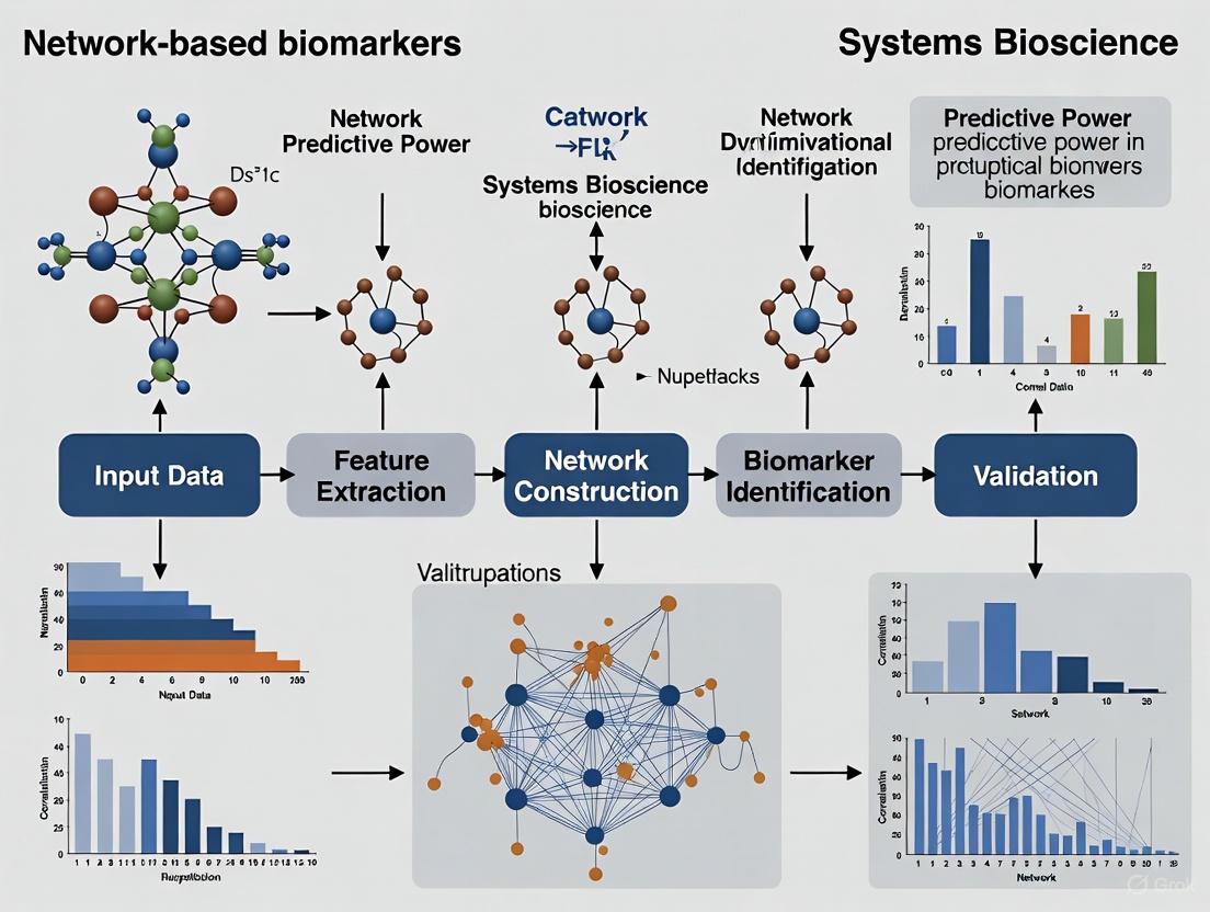
Workflow for Predictive Biomarker Identification. This diagram outlines the key steps in a network-based biomarker discovery pipeline, from data input and network construction through to the generation of ranked candidate biomarkers using machine learning.
Multilayer Network for Dynamic Biomarkers
Dynamic Network Rewiring Across States. This multilayer network visualization illustrates how gene-gene interactions can rewire between disease states (e.g., normal vs. tumor). Gene C shows a major shift in its regulatory role, making it a strong candidate Dynamic Network Biomarker.
The integration of network topology into biomarker discovery provides a powerful, biologically rational framework that transcends the limitations of reductionist approaches. By considering a biomolecule's position, connectivity, and dynamic behavior within interaction networks, researchers can prioritize candidates with a higher likelihood of clinical predictive power. This paradigm, supported by robust computational tools and validated by successful applications across cancer types, promises to accelerate the development of more effective companion diagnostics and improve patient stratification for targeted therapies.
The discovery of predictive biomarkers is being transformed by computational methods that analyze the intricate architecture of biological systems. Traditional, hypothesis-driven approaches often overlook the complex molecular interactions that dictate disease progression and treatment response. The integration of network science and machine learning provides a powerful, systems-level framework for identifying robust biomarkers. This paradigm shift leverages key network properties—network motifs, centrality measures, and the presence of intrinsically disordered proteins (IDPs)—to pinpoint molecules with critical roles in cellular information flow and signaling fidelity. These properties help elucidate why certain proteins are more likely to function as successful biomarkers, as they often occupy privileged, information-rich positions within the cellular interactome and possess unique structural characteristics that facilitate versatile interactions [4] [10] [11]. Framing biomarker discovery within this context moves the field beyond single-molecule associations towards an understanding of the disrupted system, ultimately enhancing the predictive power for patient-specific therapeutic outcomes.
Foundational Network Properties and Their Biological Significance
Network Motifs as Functional Hotspots
Network motifs are small, recurring circuit patterns within a larger network that appear more frequently than in random networks. They are considered the fundamental functional modules and building blocks of complex biological networks [10]. In transcriptional regulatory networks (TRNs), the Feed-Forward Loop (FFL), a three-node motif, is a statistically significant and well-characterized example [10]. Motifs like FFLs are not just structural artifacts; they confer specific dynamic properties to the network. They can act as filters for transient signals, generate pulse-like responses, accelerate response times, and provide robustness against network perturbations [4] [10]. From a biomarker perspective, proteins that co-participate in motifs with a drug target are enmeshed in a tight regulatory relationship, making their state a potential indicator of pathway activity and, consequently, drug response [4].
Centrality Measures for Identifying Key Players
Centrality analysis provides quantitative metrics to rank nodes (e.g., proteins or genes) based on their topological importance within a network. Identifying these "key players" is crucial for biomarker prioritization, as they are often essential for network stability and information flow [12] [13]. Different centrality measures capture distinct aspects of a node's importance:
- Degree Centrality: The number of direct connections a node has. It is a simple measure of local influence, where hubs (high-degree nodes) were initially thought to be universally essential [12] [13].
- Betweenness Centrality: Quantifies how often a node lies on the shortest path between other nodes. Nodes with high betweenness act as critical gatekeepers of information flow [12] [13].
- Closeness Centrality: Measures how quickly a node can reach all other nodes in the network via shortest paths. Nodes with high closeness can rapidly disseminate or receive information [12] [13].
- Eigenvector Centrality: A more sophisticated measure where a node's importance is determined by both its own connections and the importance of its neighbors [12].
No single centrality measure is perfect, and their performance can vary across different biological contexts. Studies have shown that combining multiple centrality measures often yields more reliable predictions of essential genes than any single measure alone [12].
Intrinsic Disorder and Network Regulation
Intrinsically Disordered Proteins (IDPs) or regions lack a stable tertiary structure under physiological conditions. This structural flexibility allows them to interact with multiple diverse partners and act as hubs in protein interaction networks [4]. IDPs are enriched in signaling and regulatory networks, where their plasticity is advantageous for facilitating new connections and integrating information from different pathways [4]. Their overrepresentation in three-nodal triangles with oncotherapeutic targets suggests a close regulatory connection, making them compelling candidates for predictive biomarkers. The presence of intrinsic disorder can be predicted computationally using tools like IUPred and AlphaFold (via per-residue confidence metrics, pLDDT), or curated from databases like DisProt [4].
Table 1: Key Network Properties and Their Biomarker Relevance
| Network Property | Biological Significance | Role in Biomarker Function |
|---|---|---|
| Network Motifs (e.g., FFLs) | Information-processing modules; provide robustness, signal filtering, and specific temporal dynamics [10]. | Indicate tight co-regulation; a neighbor's state in a motif can predict target pathway activity and drug response [4]. |
| Centrality Measures | Identify topologically essential nodes for network connectivity and information flow [12] [13]. | Prioritize proteins whose perturbation has widespread network consequences, correlating with essentiality and potential biomarker value [11]. |
| Intrinsic Disorder | Confers binding promiscuity and structural flexibility; enriched in regulatory hubs [4]. | IDPs are often critical network connectors; their state or expression can be a sensitive indicator of network rewiring in disease [4]. |
Quantitative Insights from Recent Studies
Recent research provides quantitative evidence supporting the integration of these network properties for biomarker discovery. The MarkerPredict framework, which integrates network motifs and protein disorder, classified 3,670 target-neighbor pairs using machine learning models (Random Forest and XGBoost), achieving a high leave-one-out cross-validation (LOOCV) accuracy range of 0.7 to 0.96 [4]. This study defined a Biomarker Probability Score (BPS) and identified 2,084 potential predictive biomarkers for targeted cancer therapeutics, 426 of which were classified as biomarkers by all four calculation methods [4].
Furthermore, the analysis of three signaling networks (CSN, SIGNOR, ReactomeFI) revealed that triangles containing both an IDP and a drug target member were significantly enriched, occurring with a much larger frequency than by random chance. Unbalanced triangles were particularly overrepresented among these IDP-target pairs [4]. Text-mining annotations from the CIViCmine database showed that in these networks, more than 86% of the IDPs were also annotated as prognostic biomarkers, underscoring their clinical relevance [4].
Table 2: Performance Metrics of a Network-Based Biomarker Discovery Framework (MarkerPredict) [4]
| Metric | Value / Range | Description / Context |
|---|---|---|
| LOOCV Accuracy | 0.7 - 0.96 | Performance of 32 different ML models across three signaling networks. |
| Target-Neighbor Pairs Classified | 3,670 | Total number of protein pairs evaluated. |
| Potential Biomarkers Identified | 2,084 | Biomarkers with a defined Biomarker Probability Score (BPS). |
| High-Confidence Biomarkers | 426 | Biomarkers classified positively by all 4 calculation methods. |
| IDPs as Prognostic Biomarkers | >86% | Percentage of Intrinsically Disordered Proteins annotated as prognostic biomarkers in CIViCmine. |
Experimental Protocols for Network-Based Biomarker Discovery
Protocol 1: Identifying and Analyzing Motif-Central Biomarkers
This protocol outlines the steps to discover biomarker candidates by analyzing proteins that participate in network motifs with known drug targets.
Workflow Overview:
Materials & Reagents:
- Signaling Network Data: Curated network files from sources like the Human Cancer Signaling Network (CSN), SIGNOR, or ReactomeFI [4].
- Motif Detection Software: FANMOD or an equivalent tool for enumerating network motifs [4] [10].
- Drug Target List: A curated list of proteins that are targets of known therapeutics.
- Biomarker Database: CIViCmine or similar for annotating known biomarker functions [4].
- IDP Prediction Tools: IUPred34 and/or AlphaFold33 (for pLDDT scores) to identify intrinsically disordered regions [4].
Procedure:
- Network Curation: Obtain and pre-process the chosen signaling network. Ensure the network is represented as a directed graph where possible, as link direction is crucial for motif definition.
- Motif Detection: Run the motif detection tool (e.g., FANMOD) to identify all instances of three-node motifs (specifically triangles) within the network. Statistical analysis (e.g., Z-score) should be performed to confirm the motifs are significantly over-represented compared to randomized networks [4] [10].
- Target-Motif Overlap: Cross-reference the list of drug targets with the proteins participating in the identified motifs. Create a set of "target-neighbor pairs," which are proteins that share a motif with a drug target [4].
- Biomarker Annotation: Annotate the target-neighbor pairs using a biomarker database like CIViCmine. This step establishes a ground-truth set of known predictive biomarkers (positive controls) and non-biomarkers (negative controls) for model training [4].
- Feature Engineering: For each target-neighbor pair, compute a set of features that will be used for machine learning. This should include:
- Motif-based features: The number and type of shared motifs.
- Topological features: Centrality measures (degree, betweenness) of the neighbor protein.
- Structural features: Intrinsic disorder scores from IUPred or AlphaFold for the neighbor protein [4].
- Model Training and Validation: Train a binary classifier (e.g., Random Forest or XGBoost) on the annotated dataset. Use rigorous validation methods like Leave-One-Out Cross-Validation (LOOCV) or k-fold cross-validation to assess model performance and avoid overfitting [4].
- Biomarker Prioritization: Apply the trained model to uncharacterized target-neighbor pairs. Use a composite score, like the Biomarker Probability Score (BPS), to rank the predictions and generate a final list of high-confidence biomarker candidates [4].
Protocol 2: A Multi-Layer Consensus Approach for Biomarker Prioritization
This protocol uses an ensemble of functional data to build a robust sub-network from which hub genes (potential biomarkers) are identified via centrality analysis.
Workflow Overview:
Materials & Reagents:
- Gene Expression Data: A disease-relevant transcriptomic dataset (e.g., from NCBI GEO).
- Module Detection Algorithms: A set of different algorithms (e.g., WGCNA, EXPANDER, CLICK) to identify co-expression modules [11].
- Ontological Data: Gene Ontology (GO) databases for functional annotation.
- Network Analysis Platform: Software like Cytoscape for visualization and analysis.
Procedure:
- Data Collection and Preprocessing: Obtain a disease-specific gene expression dataset (e.g., from NCBI GEO). Normalize and preprocess the data to remove technical artifacts and batch effects [11].
- Functional Module Detection: Apply multiple, independent module detection algorithms to the preprocessed expression data. This identifies groups of genes with highly correlated expression patterns, which often represent functional units [11].
- Build Consensus Networks:
- Consensus Co-expression Network: For the genes present in the top-ranked functional modules from step 2, generate a co-expression network. Use an ensemble of network inference methods to create a robust, consensus network that is less dependent on any single algorithm [11].
- Consensus Ontological Network: For the same set of genes, build a network where edges represent shared functional annotations from multiple Gene Ontology terms (e.g., Biological Process, Molecular Function, Cellular Component) [11].
- Create Final Confidence Network: Merge the consensus co-expression network and the consensus ontological network to form a single, functional confidence network. This network integrates both statistical correlation and prior biological knowledge [11].
- Centrality Analysis: Calculate multiple centrality measures (e.g., degree, betweenness, closeness) for all nodes in the confidence network.
- Hub Gene Identification: Rank the genes based on their centrality values. The top-ranked hub genes in this disease-specific, functionally-validated network are high-priority candidates for further validation as disease biomarkers or drug targets [11].
Table 3: Key Research Reagents and Computational Tools for Network-Based Biomarker Discovery
| Category / Item | Specific Examples | Function and Application |
|---|---|---|
| Signaling Network Databases | Human Cancer Signaling Network (CSN), SIGNOR, ReactomeFI [4] | Provide curated maps of protein-protein interactions and signaling pathways for network construction. |
| Motif Analysis Tools | FANMOD [4] [10] | Enumerates and identifies over-represented network motifs within a larger network structure. |
| Centrality Analysis Software | Cytoscape with plugins, NetworkX [11] [13] | Platforms for calculating a wide array of centrality measures and other topological parameters. |
| IDP Prediction Resources | IUPred34, AlphaFold33 (pLDDT), DisProt database [4] | Predict or catalog intrinsically disordered regions in protein sequences. |
| Biomarker Annotation Databases | CIViCmine [4] | Text-mined and curated database linking genes and variants to clinical evidence in cancer. |
| Module Detection Algorithms | WGCNA, EXPANDER, CLICK [11] | Identify functional modules (groups of co-expressed/co-regulated genes) from expression data. |
| Machine Learning Frameworks | Scikit-learn (Random Forest), XGBoost [4] | Provide libraries for building and validating classification models to rank biomarker candidates. |
Integrated Analysis and Future Directions
The convergence of motifs, centrality, and intrinsic disorder provides a multi-faceted lens through which to view and discover predictive biomarkers. Proteins that score highly across these dimensions—such as a hub protein with high betweenness centrality that is also an IDP and participates in multiple regulatory motifs with a drug target—are exceptionally strong candidates. Frameworks like MarkerPredict and PRoBeNet demonstrate the tangible power of this integrated approach, showing that machine learning models built on these network features significantly outperform models using randomly selected genes or all genes, especially when data is limited [4] [3].
Future research directions will likely involve a deeper integration of multi-omics data and more sophisticated temporal network analysis to capture the dynamic rewiring of biological systems in disease and treatment. Furthermore, the push for explainable AI in this field is critical for building clinical trust and generating biologically interpretable insights [14] [15]. As these methodologies mature, network-based biomarker discovery will become an indispensable component of precision medicine, enabling more accurate prediction of treatment response and improving patient outcomes in complex diseases.
Application Note: Leveraging Network-Based Predictive Biomarkers in Oncology
Therapeutic resistance and patient heterogeneity represent the most significant challenges in modern oncology. Tumor heterogeneity, both between patients (inter-tumor) and within a single tumor (intra-tumor), drives differential treatment responses and ultimately leads to therapy resistance [16] [17]. The diverse and heterogeneous nature of cancer is a fundamental characteristic responsible for therapy resistance, progression, and disease recurrence [16]. To address this clinical imperative, network-based frameworks that integrate multi-omics data, protein-protein interaction networks, and machine learning have emerged as powerful tools for discovering predictive biomarkers that can guide personalized treatment strategies.
Quantitative Landscape of Predictive Biomarkers in Oncology
Table 1: Performance Metrics of Network-Based Biomarker Discovery Platforms
| Platform Name | Algorithm(s) Used | Validation Performance (AUC) | Key Biomarkers Identified | Clinical Application |
|---|---|---|---|---|
| MarkerPredict [4] | Random Forest, XGBoost | 0.7-0.96 (LOOCV) | 426 high-confidence biomarkers across 3670 target-neighbor pairs | Predictive biomarker identification for targeted therapies |
| PRoBeNet [3] | Network propagation + ML | Significant outperformance vs. random genes | Biomarkers for infliximab response in ulcerative colitis | Autoimmune disease therapy selection |
| GTR-ITH Radiomics [17] | Multiple ML ensemble | 0.94 (training), 0.83 (test) | 17 global tumor region + 27 heterogeneity features | HCC response to TACE-ICI-MTT therapy |
Table 2: Biomarker Classification and Clinical Utility
| Biomarker Category | Definition | Key Examples | Clinical Utility |
|---|---|---|---|
| Predictive [15] | Determines likelihood of response to specific treatment | HER2 (breast cancer), EGFR mutations (lung cancer), PD-L1 | Guides targeted therapy and immunotherapy selection |
| Prognostic [15] | Indicates disease outcome independent of treatment | Ki67 (breast cancer), Oncotype DX Recurrence Score | Assesses disease aggressiveness and recurrence risk |
| Diagnostic [18] | Identifies presence and type of cancer | PSA (prostate cancer), CA-125 (ovarian cancer) | Facilitates early detection and cancer classification |
Network-Based Frameworks for Addressing Therapy Resistance
Network medicine approaches have demonstrated significant promise in unraveling the complexity of therapy resistance. The PRoBeNet framework operates on the hypothesis that the therapeutic effect of a drug propagates through a protein-protein interaction network to reverse disease states [3]. This approach prioritizes biomarkers by considering: (1) therapy-targeted proteins, (2) disease-specific molecular signatures, and (3) an underlying network of interactions among cellular components (the human interactome) [3]. Machine learning models using PRoBeNet biomarkers significantly outperformed models using either all genes or randomly selected genes, especially when data were limited.
Similarly, MarkerPredict employs network motifs and protein disorder to explore their contribution to predictive biomarker discovery [4]. The platform utilizes intrinsically disordered proteins (IDPs) enriched in network triangles as potential predictive biomarkers, as these structural features may shape their biomarker potential. MarkerPredict classified 3670 target-neighbor pairs with 32 different models achieving a 0.7-0.96 LOOCV accuracy and identified 2084 potential predictive biomarkers to targeted cancer therapeutics [4].
Imaging Biomarkers for Decoding Tumor Heterogeneity
Radiomic biomarkers have emerged as powerful non-invasive tools for quantifying intratumor heterogeneity (ITH). A recent multicenter cohort study developed a composite GTR-ITH score integrating both global tumor region and ITH-related features extracted from pre-treatment computed tomography scans [17]. This approach demonstrated high discriminative performance in predicting treatment response to transarterial chemoembolization combined with immune checkpoint inhibitor plus molecular targeted therapy (TACE-ICI-MTT) in hepatocellular carcinoma patients, with AUCs of 0.94 in the training set and 0.83 in independent testing [17]. The GTR-ITH low-risk group exhibited an immune-inflamed microenvironment characterized by enriched plasma cells and M1 macrophages, and reduced M2 macrophage infiltration, providing biological relevance to the imaging biomarkers.
Experimental Protocols
Protocol 1: Network-Based Biomarker Discovery Using MarkerPredict
Principle and Scope
This protocol describes the methodology for identifying predictive biomarkers using the MarkerPredict framework, which integrates network motifs, protein disorder, and machine learning to predict clinically relevant biomarkers for targeted cancer therapies [4]. The approach is based on the observation that intrinsically disordered proteins are enriched in network triangles and are likely to be cancer biomarkers.
Materials and Reagents
Table 3: Research Reagent Solutions for Network-Based Biomarker Discovery
| Item | Specification/Function | Example Sources/Platforms |
|---|---|---|
| Signaling Networks | Human Cancer Signaling Network (CSN), SIGNOR, ReactomeFI | [4] |
| IDP Databases | DisProt, AlphaFold (pLLDT<50), IUPred (score > 0.5) | [4] |
| Biomarker Annotation | CIViCmine text-mining database | [4] |
| Machine Learning Frameworks | Random Forest, XGBoost (Python implementations) | [4] |
| Motif Identification | FANMOD programme | [4] |
Procedure
Step 1: Network Motif Identification and Triangle Selection
- Obtain three signed subnetworks from Human Cancer Signaling Network (CSN), SIGNOR, and ReactomeFI
- Identify three-nodal motifs using FANMOD programme
- Select fully connected three-nodal motifs (triangles) for analysis, with special attention to unbalanced triangles (with odd number of negative links) and cycles
- Confirm enrichment of triangles containing both DisProt IDP and target members compared to random chance
Step 2: Training Dataset Construction
- Annotate biomarker properties using CIViCmine text-mining database
- Establish positive controls (class 1): cases where disordered protein was the predictive biomarker for its target triangle pair (332 cases of 4550 neighbor-target pairs)
- Establish negative control dataset from neighbor proteins not present in CIViCmine and random pairs
- Create final training set of 880 target-interacting protein pairs total
Step 3: Machine Learning Model Training and Optimization
- Implement both Random Forest and XGBoost binary classification methods
- Train on both network-specific and combined data of all 3 signaling networks
- Train on individual and combined data of all 3 IDP databases and prediction methods (32 total models)
- Set optimal hyperparameters with competitive random halving
- Perform validation using Leave-one-out-cross-validation (LOOCV), k-fold cross-validation, and 70:30 train-test splitting
Step 4: Biomarker Probability Score (BPS) Calculation and Classification
- Define Biomarker Probability Score as normalized summative rank of the models
- Classify 3670 target-neighbor pairs using the 32 different models
- Identify high-confidence biomarkers (426 classified as biomarker by all 4 calculations)
Protocol 2: Radiomic Biomarker Development for Tumor Heterogeneity
Principle and Scope
This protocol details the methodology for developing imaging biomarkers that capture intratumor heterogeneity (ITH) to predict treatment response in hepatocellular carcinoma (HCC) patients receiving combination therapy [17]. The approach integrates radiomic features representing both global tumor regions and ITH to create a composite biomarker score.
Materials and Reagents
- Pre-treatment computed tomography scans from multicenter cohort
- Radiomic feature extraction software (Python-based radiomics packages)
- Bulk RNA sequencing data from The Cancer Imaging Archive for biological validation
- Multiple machine learning algorithms for ensemble learning
- Principal component analysis tools for feature integration
Procedure
Step 1: Patient Cohort Selection and Image Acquisition
- Include patients with unresectable HCC receiving first-line TACE-ICI-MTT
- Ensure consistent CT imaging protocols across multiple centers
- Curate clinical data including treatment response and survival outcomes
Step 2: Radiomic Feature Extraction and Selection
- Extract features representing global tumor regions (GTR) and intratumor heterogeneity (ITH)
- Perform feature selection to retain most informative features (17 GTR-related and 27 ITH-related features)
- Generate composite GTR-ITH score using principal component analysis
Step 3: Machine Learning Model Development and Validation
- Employ ensemble learning with multiple machine learning algorithms
- Divide data into training, internal validation, and independent test sets
- Evaluate model performance by area under the receiver operating characteristic curve (AUC)
- Validate survival prediction using Kaplan-Meier analysis and log-rank test
Step 4: Biological Validation and Microenvironment Characterization
- Characterize immune infiltration patterns using bulk RNA sequencing data
- Correlate GTR-ITH score with immune microenvironment phenotypes
- Confirm immune-inflamed microenvironment in GTR-ITH low-risk group (enriched plasma cells and M1 macrophages, reduced M2 macrophage infiltration)
Protocol 3: PRoBeNet Framework for Predictive Biomarker Discovery
Principle and Scope
This protocol describes the PRoBeNet (Predictive Response Biomarkers using Network medicine) framework for discovering treatment-response-predicting biomarkers for complex diseases [3]. The method operates under the hypothesis that the therapeutic effect of a drug propagates through a protein-protein interaction network to reverse disease states.
Materials and Reagents
- Protein-protein interaction network (human interactome)
- Disease-specific molecular signatures
- Therapy-targeted proteins information
- Gene expression data from patient cohorts
- Machine learning frameworks for model building
Procedure
Step 1: Network Construction and Data Integration
- Compile comprehensive human interactome (protein-protein interaction network)
- Integrate disease-specific molecular signatures
- Incorporate therapy-targeted proteins information
Step 2: Biomarker Prioritization
- Prioritize biomarkers based on network proximity to therapy targets
- Consider network propagation of therapeutic effects
- Identify key nodes that reverse disease states when targeted
Step 3: Model Validation with Retrospective and Prospective Data
- Validate predictive power with retrospective gene-expression data from patients with ulcerative colitis and rheumatoid arthritis
- Perform prospective validation with tissues from patients with ulcerative colitis and Crohn disease
- Compare performance against models using all genes or randomly selected genes
Step 4: Clinical Translation
- Develop companion and complementary diagnostic assays
- Stratify suitable patient subgroups for clinical trials
- Implement biomarkers for improved patient outcomes
The Scientist's Toolkit: Essential Research Reagent Solutions
Table 4: Key Research Reagent Solutions for Biomarker Discovery
| Category | Specific Items | Function/Application | Key References |
|---|---|---|---|
| Network Databases | Human Cancer Signaling Network (CSN), SIGNOR, ReactomeFI | Provide signed signaling networks for motif analysis and biomarker discovery | [4] |
| IDP Resources | DisProt, AlphaFold (pLLDT<50), IUPred (score > 0.5) | Identify intrinsically disordered proteins with biomarker potential | [4] |
| Biomarker Annotation | CIViCmine text-mining database | Annotate biomarker properties and establish training sets | [4] |
| Machine Learning Platforms | Random Forest, XGBoost, Ensemble Methods | Develop predictive models for biomarker classification | [4] [17] |
| Imaging Biomarker Tools | Radiomic feature extraction software, PCA tools | Quantify intra-tumor heterogeneity and global tumor characteristics | [17] |
| Validation Resources | Bulk RNA sequencing, Immune profiling assays | Biological validation of biomarker associations with microenvironment | [17] |
Methodologies in Action: Machine Learning and Network Algorithms for Biomarker Identification
The advancement of precision medicine relies heavily on the identification of robust predictive biomarkers to guide therapeutic decisions, particularly in complex diseases like cancer and autoimmune disorders. Traditional methods for biomarker discovery often face challenges of limited data availability and inadequate sample sizes when compared to the high dimensionality of molecular data. Computational frameworks that leverage network biology principles have emerged as powerful tools to address these limitations. By integrating protein-protein interaction networks, multi-omics data, and machine learning algorithms, these frameworks can systematically prioritize biomarker candidates with higher predictive potential. This article explores three prominent computational frameworks—PRoBeNet, MarkerPredict, and Comparative Network Stratification (CNS)—that utilize network-based approaches to discover biomarkers with predictive power for treatment response. These frameworks represent a paradigm shift from reductionist approaches to systems-level analyses that capture the complex interplay within biological systems, potentially offering more clinically relevant biomarkers for personalized treatment strategies.
The PRoBeNet Framework
Conceptual Foundation and Methodology
PRoBeNet (Predictive Response Biomarkers using Network medicine) is a novel framework developed to address the challenge of limited data availability in precision medicine for complex autoimmune diseases. This framework operates on the core hypothesis that the therapeutic effect of a drug propagates through a protein-protein interaction network to reverse disease states [3]. Unlike conventional approaches that focus solely on differential expression, PRoBeNet employs a more sophisticated strategy that prioritizes biomarkers by considering three critical elements: (1) therapy-targeted proteins, (2) disease-specific molecular signatures, and (3) an underlying network of interactions among cellular components (the human interactome) [3].
The methodology involves mapping both disease signatures and drug targets onto a comprehensive human interactome network. The framework then identifies proteins that occupy strategic positions in the network relative to both disease processes and drug mechanisms. These proteins are considered strong candidates for predictive biomarkers because they potentially mediate or reflect the propagation of therapeutic effects through biological networks. Validation studies have demonstrated that PRoBeNet successfully discovered biomarkers predicting patient responses to both established autoimmune therapies (infliximab) and investigational compounds (a mitogen-activated protein kinase 3/1 inhibitor) [3].
Experimental Protocol and Implementation
Protocol: PRoBeNet Biomarker Discovery
Step 1: Data Collection and Curation
- Compile a comprehensive human protein-protein interaction (PPI) network from reference databases (e.g., STRING, BioGRID).
- Obtain disease-specific molecular signatures from transcriptomic studies of patient tissues.
- Curate a list of therapy-targeted proteins based on drug mechanism of action studies.
Step 2: Network Integration and Analysis
- Map disease signatures and drug targets onto the PPI network.
- Implement network propagation algorithms to simulate the spread of therapeutic effects from drug targets.
- Identify proteins within the network that show significant proximity to both disease-associated regions and drug targets.
Step 3: Biomarker Prioritization
- Rank candidate biomarkers based on their network topological properties (e.g., centrality, proximity to targets).
- Apply machine learning models built specifically with PRoBeNet-identified features.
- Validate predictive power using retrospective gene-expression data from patient cohorts.
Step 4: Experimental Validation
- Verify top biomarker candidates in prospective clinical samples using appropriate molecular assays (e.g., RT-qPCR, RNA-seq).
- Assess the clinical utility of biomarkers for patient stratification in relevant therapeutic contexts.
The framework has shown particular strength in constructing robust machine-learning models when data are limited, significantly outperforming models using either all genes or randomly selected genes [3]. This makes PRoBeNet especially valuable for biomarker discovery in rare diseases or patient subgroups where large sample sizes are difficult to obtain.
PRoBeNet Workflow Visualization
The MarkerPredict Framework
Conceptual Foundation and Methodology
MarkerPredict is a specialized computational framework designed specifically for predicting clinically relevant predictive biomarkers for targeted cancer therapies [4]. This approach integrates two key biological concepts that shape biomarker potential: network-based properties of proteins and structural features such as intrinsic disorder [4]. The framework is founded on the observation that intrinsically disordered proteins (IDPs) are significantly enriched in three-nodal network motifs (triangles) with oncotherapeutic targets, suggesting a close regulatory relationship that may be exploitable for biomarker development [4].
The methodology employs machine learning to classify target-neighbour pairs based on their potential as predictive biomarkers. MarkerPredict was trained on literature evidence-based positive and negative training sets comprising 880 target-interacting protein pairs total using both Random Forest and XGBoost algorithms across three different signaling networks [4]. The framework achieved impressive performance metrics, with Leave-One-Out-Cross-Validation (LOOCV) accuracy ranging from 0.7 to 0.96 across 32 different models [4]. To facilitate biomarker prioritization, MarkerPredict introduces a Biomarker Probability Score (BPS), defined as a normalized summative rank of the models, which enables quantitative assessment and ranking of potential biomarkers [4].
Experimental Protocol and Implementation
Protocol: MarkerPredict Biomarker Prediction
Step 1: Data Collection and Feature Extraction
- Collect three signaling networks: Human Cancer Signaling Network (CSN), SIGNOR, and ReactomeFI.
- Identify three-nodal motifs (triangles) using the FANMOD programme.
- Calculate network topological properties for all proteins (centrality, participation in motifs).
- Annotate intrinsic disorder using multiple databases/methods: DisProt, AlphaFold (pLLDT<50), and IUPred (score > 0.5).
Step 2: Training Set Construction
- Create positive controls from established predictive biomarker-target pairs (332 pairs annotated from CIViCmine database).
- Compile negative controls from neighbor proteins not present in CIViCmine and random pairs.
- Manually review and curate the final training set of 880 protein pairs.
Step 3: Machine Learning Model Development
- Implement both Random Forest and XGBoost algorithms.
- Train models on both network-specific and combined data across all three signaling networks.
- Optimize hyperparameters using competitive random halving.
- Validate models using LOOCV, k-fold cross-validation, and 70:30 train-test splitting.
Step 4: Biomarker Classification and Scoring
- Apply trained models to classify 3,670 target-neighbour pairs.
- Calculate Biomarker Probability Score (BPS) as normalized average of ranked probability values.
- Prioritize candidates based on BPS for experimental validation.
Application of MarkerPredict identified 2,084 potential predictive biomarkers for targeted cancer therapeutics, with 426 classified as biomarkers by all four calculations [4]. The framework has been specifically used to detail the biomarker potential of LCK and ERK1 in cancer therapeutics, demonstrating its utility for generating clinically relevant hypotheses [4].
MarkerPredict Workflow Visualization
Comparative Network Stratification (CNS)
Conceptual Foundation
Comparative Network Stratification (CNS) is a computational framework designed for patient stratification through comparative analysis of molecular networks across patient subgroups. While detailed methodology for CNS was not available in the search results, the approach generally involves constructing disease-specific networks for different patient subgroups and identifying differential network regions that correspond to distinct disease mechanisms or treatment responses. This framework is particularly valuable for addressing disease heterogeneity, which often undermines the development of universally effective biomarkers and therapies.
CNS typically integrates multi-omics data to construct comprehensive molecular networks that capture the complex interactions within biological systems. By comparing these networks across patient populations with different clinical outcomes, the framework can identify network-based subtypes that may respond differently to treatments. This approach aligns with the broader trend in precision medicine toward moving beyond traditional biomarkers to network-based stratification that better reflects the complexity of disease mechanisms.
Comparative Analysis of Frameworks
Framework Comparison Table
The following table provides a detailed comparison of the key features, methodologies, and applications of PRoBeNet, MarkerPredict, and CNS:
| Feature | PRoBeNet | MarkerPredict | CNS |
|---|---|---|---|
| Primary Application | Predicting response biomarkers for complex autoimmune diseases [3] | Predicting predictive biomarkers for targeted cancer therapies [4] | Patient stratification through network comparison |
| Core Methodology | Network propagation from drug targets through interactome | Machine learning on network motifs and protein disorder features [4] | Comparative analysis of molecular networks across subgroups |
| Network Types | Protein-protein interaction networks | Signaling networks (CSN, SIGNOR, ReactomeFI) [4] | Disease-specific molecular networks |
| Key Biological Features | Drug targets, disease signatures, network proximity | Intrinsic disorder, network motif participation [4] | Multi-omics patterns, network topology |
| Machine Learning Approach | Models using PRoBeNet-selected features | Random Forest & XGBoost (32 models) [4] | Not specified in available sources |
| Validation Methods | Retrospective & prospective gene-expression data [3] | LOOCV, k-fold CV, train-test split (0.7-0.96 accuracy) [4] | Not specified in available sources |
| Key Output | Prioritized predictive biomarkers | Biomarker Probability Score (BPS) [4] | Patient subgroups, network subtypes |
| Unique Strength | Effective with limited data; reduces features for robust models [3] | Integrates structural disorder with network topology [4] | Addresses disease heterogeneity |
Performance Metrics Table
The following table summarizes the performance characteristics and validation results for the frameworks:
| Performance Aspect | PRoBeNet | MarkerPredict | CNS |
|---|---|---|---|
| Reported Accuracy | Significantly outperforms all-gene or random-gene models [3] | LOOCV accuracy: 0.7-0.96 across models [4] | Not available |
| Data Efficiency | Works well with limited data samples [3] | Requires sufficient training pairs (880 in original) [4] | Not available |
| Validation Evidence | Retrospective data from UC, RA; prospective from CD [3] | Classification of 3,670 pairs; 426 high-confidence biomarkers [4] | Not available |
| Clinical Translation | Potential for companion diagnostics [3] | Encourages clinical validation [4] | Not available |
| Scalability | Suitable for multi-omics integration | Can scale with network size and disorder data | Not available |
The Scientist's Toolkit
Successful implementation of network-based biomarker discovery frameworks requires specific computational tools and biological resources. The following table details essential components of the research toolkit for these approaches:
| Resource Type | Specific Tools/Databases | Function in Research |
|---|---|---|
| Signaling Networks | Human Cancer Signaling Network (CSN), SIGNOR, ReactomeFI [4] | Provide curated biological networks for analysis and feature extraction |
| IDP Databases | DisProt, IUPred, AlphaFold [4] | Annotate intrinsic protein disorder, a key feature in MarkerPredict |
| Biomarker Databases | CIViCmine [4] | Provide validated biomarker information for training and validation |
| Motif Detection | FANMOD programme [4] | Identify network motifs (triangles) for feature calculation |
| Machine Learning | Random Forest, XGBoost [4] | Implement classification algorithms for biomarker prediction |
| Implementation | PRoBeNet framework, MarkerPredict (GitHub) [4] [3] | Ready-to-use computational frameworks for biomarker discovery |
| Validation Data | Retrospective gene-expression data from patient cohorts [3] | Validate predictive power of discovered biomarkers |
Network-based computational frameworks represent a powerful paradigm shift in predictive biomarker discovery. PRoBeNet, MarkerPredict, and CNS each offer distinct approaches to addressing the fundamental challenge of connecting biological complexity to clinically actionable predictions. While PRoBeNet excels in contexts with limited data availability and MarkerPredict offers specialized capability for cancer therapeutics by integrating structural disorder, CNS focuses on addressing disease heterogeneity through comparative network analysis.
The future development of these frameworks will likely involve several key directions: First, increased integration of multi-omics data will provide more comprehensive biological context for predictions. Second, improvement in interpretability methods will enhance clinical translation by providing mechanistic insights alongside predictions. Third, incorporation of temporal dynamics through longitudinal data analysis may capture the evolving nature of treatment responses. Finally, standardization of validation protocols across frameworks will facilitate comparative assessment and clinical adoption.
As these frameworks mature, they hold significant promise for transforming precision medicine by enabling more accurate prediction of treatment responses, ultimately leading to improved patient outcomes and more efficient therapeutic development.
Within the paradigm of network medicine, diseases are rarely caused by single gene defects but rather arise from perturbations in complex cellular networks. Network propagation has emerged as a powerful computational technique that leverages protein-protein interaction (PPI) networks to identify biomarkers and therapeutic targets by simulating the flow of information from known disease-associated genes. This approach is grounded in the "guilt-by-association" principle, wherein proteins proximal to known targets in the network are likely involved in related biological processes and disease mechanisms. By framing biomarker discovery within the context of a broader thesis on network-based biomarkers' predictive power, this protocol details practical methodologies for implementing network propagation to uncover biomarkers proximal to drug targets, thereby accelerating therapeutic development.
The core hypothesis is that genes causing similar phenotypes tend to interact with one another, and that the functional influence of a gene or protein extends to its network neighbors. Network-based methods systematically contextualize individual molecular entities within the broader cellular system, moving beyond differential expression alone to identify biomarkers based on their topological significance. This is particularly valuable for understanding complex drug response mechanisms, as resistance is often mediated through alternative pathways that bypass the primary drug target [19].
Quantitative Foundations of Network Propagation
The application of network propagation relies on several key quantitative metrics and algorithms that determine how "influence" spreads through a network. The following table summarizes the core computational components.
Table 1: Core Algorithms and Metrics in Network Propagation
| Component | Algorithm/Metric | Function in Biomarker Identification | Key Formula/Parameters |
|---|---|---|---|
| Network Propagation | PageRank / Random Walk with Restart | Prioritizes genes based on their proximity and connectivity to known seed genes (e.g., drug targets) in the PPI network. | ( PR(gi; t) = \frac{1-d}{N} + d \sum{gj \in B(gi)} \frac{PR(gj; t-1)}{L(gj)} ) Where (d) is a damping factor, (B(gi)) are neighbors, and (L(gj)) is the out-degree [20]. |
| Path Analysis | k-Shortest Paths (PathLinker) | Identifies critical communication pathways between proteins, revealing potential bypass routes used in drug resistance. | Parameter k (e.g., 200) defines the number of shortest simple paths to compute between source and target nodes [19]. |
| Centrality Analysis | Betweenness, Closeness, Degree | Quantifies the topological importance of a node within the network, helping to identify bottleneck proteins or key connectors. | Integrated into frameworks like BEERE for iterative gene list ranking and expansion [21]. |
| Statistical Enrichment | Hypergeometric Test | Determines if a set of candidate genes is significantly over-represented in a specific biological pathway, adding functional context. | Used to map candidate genes to ICI-related pathways [20]. |
The PageRank algorithm, a cornerstone of many propagation methods, operates by iteratively distributing a "score" across the network. Seeds (e.g., known drug targets) are initialized with a high score, which is then propagated to their immediate neighbors. The damping factor d (typically ~0.85) ensures the process converges and models the probability that propagation restarts from a seed node. This process prioritizes nodes that are highly connected and close to multiple seeds, making them strong biomarker candidates [20].
The k-shortest paths approach complements this by not just looking at direct neighbors but at the ensemble of shortest paths that connect two proteins of interest, such as a drug target and a transcription factor. Analyzing these paths can reveal which intermediary proteins are most frequently used for communication within the cell. In cancer, these frequently used intermediaries can represent vulnerabilities whose targeting can block resistance mechanisms [19].
Application Note: Predictive Biomarker Discovery for Immune Checkpoint Inhibitor (ICI) Response
Background and Rationale
Predicting patient response to Immune Checkpoint Inhibitors (ICIs) remains a major challenge in oncology. While biomarkers like PD-L1 expression and tumor mutational burden are used, they lack consistent predictive power across cancer types. The PathNetDRP framework was developed to address this by identifying functionally relevant biomarkers using network propagation on PPI and pathway networks, moving beyond simple differential expression analysis [20].
Protocol: The PathNetDRP Workflow
This protocol outlines the steps for identifying and validating biomarkers for ICI response.
Table 2: PathNetDRP Protocol Workflow
| Step | Procedure | Input Data | Output |
|---|---|---|---|
| 1. Seed Initialization | Compile a list of known ICI target genes (e.g., PD-1, CTLA-4). | ICI target lists from databases like DrugBank or TTD. | Seed gene set ( S ). |
| 2. Network Propagation | Run the PageRank algorithm on a PPI network, initializing scores with seed genes ( S ). | High-confidence PPI network (e.g., from HIPPIE, STRING). | A ranked list of candidate genes influenced by the ICI targets. |
| 3. Pathway Mapping | Perform hypergeometric testing to identify biological pathways significantly enriched with the top-ranked candidate genes. | Pathway databases (e.g., KEGG, Reactome). | A set of ICI-response-related pathways ( P ). |
| 4. PathNetGene Scoring | For each pathway in ( P ), construct a pathway-specific subnetwork and re-run PageRank. Calculate the final PathNetGene Score as the mean PageRank score across all relevant pathways. | Pathway ( P ) and the PPI network. | Final prioritized list of biomarkers with PathNetGene scores. |
| 5. Validation | Use the top biomarkers as features in a machine learning classifier to predict ICI response (Responder vs. Non-Responder) on transcriptomic data from patient cohorts. | Gene expression data from ICI-treated patients (e.g., from TCGA). | A predictive model with performance metrics (AUC, accuracy). |
The following diagram illustrates the logical flow and data transformation throughout the PathNetDRP protocol.
PathNetDRP Biomarker Discovery Workflow
Outcome and Interpretation
In validation across multiple independent ICI-treated patient cohorts, PathNetDRP demonstrated a significant increase in predictive performance, with the area under the receiver operating characteristic (ROC) curve improving from 0.780 using conventional methods to 0.940 [20]. The framework not only provided a predictive gene list but also offered biological interpretability by highlighting key immune-related pathways. Researchers should prioritize biomarkers with high PathNetGene scores that also reside in pathways with known immune function (e.g., T cell signaling, cytokine-cytokine receptor interaction) for further experimental validation.
Protocol: Discovering Combinatorial Drug Targets to Overcome Resistance
Background and Rationale
A major limitation of monotherapy in oncology is the development of drug resistance, often through cancer cells activating alternative signaling pathways that bypass the inhibited target. This protocol describes a network-based strategy to discover optimal co-target combinations that preemptively block these bypass routes [19].
Detailed Experimental Methodology
Table 3: Protocol for Combinatorial Target Discovery
| Step | Activity | Specifications & Reagents |
|---|---|---|
| 1. Input Data Curation | Identify significant pairs of co-existing mutations from cancer genomics data. | Data: Somatic mutation profiles from TCGA, AACR GENIE. Tool: Fisher's Exact Test with multiple-testing correction. |
| 2. Shortest Path Calculation | For each significant mutation pair, compute the k-shortest paths in the PPI network. | Tool: PathLinker. Parameter: k = 200 (Jaccard index ~0.73 vs. k=300/400). Network: HIPPIE PPI network. |
| 3. Subnetwork Construction | Aggregate all nodes and edges from the computed shortest paths for all mutation pairs. | Output: A focused subnetwork representing key communication pathways. |
| 4. Topological Analysis | Identify key connector nodes within the subnetwork based on centrality measures. | Metrics: Betweenness centrality, degree. Focus: Proteins that serve as bridges between different mutation pairs. |
| 5. Target Prioritization & Validation | Select connector nodes from alternative pathways as co-targets. Test combinations in vitro and in vivo. | Validation: Patient-derived xenograft (PDX) models. Example: Alpelisib (PI3Ki) + LJM716 (HER3i) in breast cancer. |
The following pathway diagram visualizes the conceptual rationale behind targeting connector proteins to block resistance routes.
Network-Based Resistance and Combination Targeting
Outcome and Interpretation
Application of this protocol to patient-derived breast and colorectal cancer models successfully identified effective drug combinations. In breast cancer with ESR1/PIK3CA co-mutations, the combination of alpelisib (PI3K inhibitor) and LJM716 (HER3 inhibitor) diminished tumors. In colorectal cancer with BRAF/PIK3CA co-mutations, the triple combination of alpelisib, cetuximab (EGFR inhibitor), and encorafenib (BRAF inhibitor) showed context-dependent tumor growth inhibition [19]. The key to success is selecting co-targets that are topological connectors in the subnetwork, thereby disrupting the cancer cell's ability to re-route signals.
Successful implementation of network propagation requires a curated set of computational tools and biological datasets. The following table details essential resources.
Table 4: Key Research Reagents and Computational Resources
| Resource Name | Type | Function in Protocol | Access Link/Reference |
|---|---|---|---|
| HIPPIE PPI Database | Biological Database | Provides a high-confidence, continuously updated human protein-protein interaction network for network construction. | http://cbdm-01.zdv.uni-mainz.de/~mschaefer/hippie/ [19] |
| PathLinker | Algorithm/Software | Reconstructs signaling pathways by computing k-shortest paths between source and target proteins in a network. | https://github.com/Murali-group/PathLinker [19] |
| TCGA & AACR GENIE | Genomic Data Repository | Provides somatic mutation profiles and clinical data from thousands of cancer patients for identifying co-existing mutations. | https://www.cancer.gov/ccg/research/genome-sequencing/tcga [19] |
| Kyoto Encyclopedia of Genes and Genomes (KEGG) | Pathway Database | Curated repository of biological pathways used for functional enrichment analysis of candidate biomarkers. | https://www.genome.jp/kegg/ [20] |
| BEERE (Biological Entity Expansion and Ranking Engine) | Computational Tool | A network-based tool that uses centrality measures to iteratively rank and expand a list of candidate genes. | Described in GETgene-AI framework [21] |
This document provides detailed Application Notes and Protocols for the integrated use of Random Forest (RF), XGBoost, and Graph Neural Networks (GNNs) for classification tasks, with a specific focus on identifying predictive network-based biomarkers in oncology. This integrated approach leverages the complementary strengths of tree-based models and deep learning for enhanced feature analysis, robust classification, and improved interpretability of biological networks. The protocols outlined below have been validated in research for classifying clinically relevant biomarkers and predicting drug responses, demonstrating superior performance over single-model approaches [7] [22].
Performance Comparison of Integrated Models
The integration of these models has been systematically benchmarked across various biological and chemical datasets. The following table summarizes the typical performance metrics achieved by individual and integrated models in relevant tasks.
Table 1: Comparative Performance of ML Models in Biomedical Classification and Regression Tasks
| Model / Study | Task Description | Key Performance Metrics | Key Findings |
|---|---|---|---|
| MarkerPredict (RF & XGBoost) [7] | Classifying predictive oncological biomarkers (LOOCV) | LOOCV Accuracy: 0.7 - 0.96 | High accuracy in identifying predictive biomarker-protein pairs from signaling networks. |
| Biologically Informed NN (BINN) [22] | Stratifying septic AKI and COVID-19 subphenotypes | ROC-AUC: 0.99 ± 0.00 (AKI), 0.95 ± 0.01 (COVID-19) | Outperformed benchmarked models, including RF and XGBoost. |
| Stacking Ensemble [23] | Predicting Pharmacokinetic (PK) parameters | R²: 0.92, MAE: 0.062 | Stacking of multiple models, including GNNs and XGBoost, achieved highest accuracy. |
| GNNSeq (GNN+RF+XGBoost) [24] | Protein-ligand binding affinity prediction | Pearson CC: 0.784, R²: 0.595 | Hybrid model leveraging sequence-based features showed robust performance. |
| Descriptor-Based (SVM, XGB, RF) [25] | Molecular property prediction (11 public datasets) | Variable by dataset | On average, descriptor-based models (XGBoost, RF) outperformed graph-based models in accuracy and computational efficiency. |
Detailed Experimental Protocols
Protocol 1: Biomarker-Target Pair Classification Using Tree-Based Ensembles
This protocol is adapted from the MarkerPredict framework for identifying predictive biomarkers in cancer signaling networks using RF and XGBoost [7].
1. Objective: To classify protein-neighbor pairs in biological networks as potential predictive biomarkers for targeted cancer therapeutics.
2. Research Reagent Solutions & Materials:
- Biological Networks: Human Cancer Signaling Network (CSN), SIGNOR, or ReactomeFI networks [7].
- Biomarker Database: CIViCmine database for annotated, evidence-based biomarkers [7].
- Protein Disorder Data: DisProt, AlphaFold (pLLDT<50), or IUPred (score >0.5) databases [7].
- Software: Python with Scikit-learn and XGBoost libraries.
3. Procedure:
- Step 1: Data Compilation and Feature Engineering
- Extract all direct neighbor pairs (nodes connected by an edge) from the chosen biological network(s).
- Calculate network topological features for each node and pair (e.g., degree, betweenness centrality, clustering coefficient).
- Calculate protein-specific features, such as intrinsic disorder scores from multiple databases.
- Annotate pairs where the neighbor is a known predictive biomarker for the target drug using the CIViCmine database to create positive training labels [7].
- Step 2: Construct Training Sets
- Positive Set: Literature-validated predictive biomarker-target pairs.
- Negative Set: Protein-neighbor pairs not listed as predictive biomarkers in CIViCmine, or randomly selected non-interacting pairs [7].
- Step 3: Model Training and Validation
- Train multiple RF and XGBoost models on network-specific and combined-network data.
- Optimize hyperparameters (e.g., number of trees, max depth, learning rate) using techniques like competitive random halving [7].
- Validate models rigorously using Leave-One-Out-Cross-Validation (LOOCV), k-fold cross-validation, and a held-out test set.
- Step 4: Ranking and Interpretation
- Define a Biomarker Probability Score (BPS) as a normalized summative rank across all trained models.
- Use the BPS to rank all potential biomarker-target pairs for further biological validation [7].
The following diagram illustrates the logical workflow of this protocol:
Protocol 2: Integrating GNNs with Tree-Based Models for Enhanced Prediction
This protocol describes a hybrid approach, inspired by models like GNNSeq, which leverages the strengths of both GNNs and tree-based models for tasks such as binding affinity prediction or patient stratification [24].
1. Objective: To build a hybrid model that uses GNNs for automatic feature learning from graph-structured data and tree-based models (RF, XGBoost) for final classification/regression, improving generalizability and accuracy.
2. Research Reagent Solutions & Materials:
- Graph Data: Molecular graphs (atoms as nodes, bonds as edges) or patient similarity graphs [26] [24].
- Feature Sets: Protein sequences, ligand SMILES strings, or clinical tabular data [24].
- Software: PyTorch Geometric or Deep Graph Library (DGL) for GNNs, combined with Scikit-learn and XGBoost.
3. Procedure:
- Step 1: Graph Construction and Feature Definition
- Define the graph structure relevant to the problem.
- For molecules: Natural graph (atoms=nodes, bonds=edges).
- For patient data: Create a graph using k-NN or clustering (e.g., K-Means, HDBSCAN) on tabular features, where nodes are patients and edges represent similarity [26].
- Assign initial node features (e.g., atom type, patient clinical variables).
- Define the graph structure relevant to the problem.
- Step 2: GNN-Based Feature Learning
- Choose a GNN architecture (e.g., GCN, GAT, MPNN, GraphSAGE).
- Pass the graph through the GNN. The message-passing layers will create enriched node representations by aggregating information from neighboring nodes [27].
- Perform a readout (global pooling) on the final node embeddings to generate a fixed-size, graph-level representation vector.
- Step 3: Feature Integration and Final Prediction
- Concatenate the GNN-derived graph-level vector with other non-graph features (e.g., molecular descriptors, patient demographics).
- Feed this concatenated feature vector into a final tree-based model (RF or XGBoost) for the classification or regression task [24].
- This ensemble leverages the GNN's ability to learn complex topological patterns and the tree-based model's power in handling structured, heterogeneous data.
- Step 4: Model Validation and Interpretation
- Validate the entire pipeline using k-fold cross-validation.
- Use SHAP (SHapley Additive exPlanations) analysis on the tree-based model to interpret the contribution of both the GNN-learned features and the original features to the final prediction [25].
The following diagram illustrates the architecture of this hybrid model:
The Scientist's Toolkit: Essential Research Reagents and Materials
Table 2: Key Research Reagent Solutions for Integrated ML Pipelines
| Item Name | Function / Application | Specific Examples / Notes |
|---|---|---|
| Biological Network Databases | Provide the foundational graph structure for relationship mining and feature extraction. | Human Cancer Signaling Network (CSN) [7], SIGNOR [7], ReactomeFI [7] [22]. |
| Biomarker & Protein Databases | Source for training labels, protein features, and functional annotations. | CIViCmine (biomarker evidence) [7], DisProt (intrinsic disorder) [7], AlphaFold DB (protein structure) [7]. |
| Molecular & Compound Datasets | Benchmarking and training models for drug discovery tasks. | PDBbind (binding affinity) [24], MoleculeNet (various molecular properties) [25], ChEMBL (bioactive molecules) [23]. |
| GNN Software Libraries | Provide pre-implemented GNN architectures and graph data utilities. | PyTorch Geometric, Deep Graph Library (DGL). Supports GCN, GAT, MPNN, etc. [27] [28]. |
| Tree-Based ML Libraries | Efficient implementation of RF and gradient boosting algorithms. | Scikit-learn (RF), XGBoost library. Essential for building high-performance tabular models [7] [25]. |
| Model Interpretation Tools | Provide post-hoc explanations for complex model predictions, crucial for biological insight. | SHAP (SHapley Additive exPlanations) [22] [25]. |
Multi-omics data fusion represents a transformative approach in biomedical research, enabling a holistic understanding of biological systems by integrating complementary molecular datasets. This integrated analysis moves beyond the limitations of single-omics approaches to capture the complex interplay between different biological layers, from genetic blueprint to functional proteins. By combining genomics, transcriptomics, and proteomics data from the same set of samples, researchers can bridge the information flow from genotype to phenotype, revealing system-level insights that would otherwise remain hidden [29]. This capability is particularly valuable for identifying robust network-based biomarkers with enhanced predictive power for complex diseases, ultimately advancing the field of precision oncology and therapeutic development [4] [3].
The fundamental challenge in multi-omics integration lies in the technological and statistical complexity of combining datasets with different properties, dimensionalities, and noise structures. However, with the advent of high-throughput techniques and sophisticated computational methods, researchers can now effectively integrate these disparate datasets to uncover novel biological patterns, improve disease subtyping, and identify predictive biomarkers for treatment response [29] [30]. This protocol outlines comprehensive methodologies for fusing genomics, transcriptomics, and proteomics data, with particular emphasis on applications in network-based biomarker discovery.
Multi-Omics Integration Approaches and Protocols
Data Acquisition and Quality Control from Public Repositories
The first critical step involves acquiring high-quality multi-omics data from curated repositories. Several consortia provide comprehensive molecular datasets with matched samples across multiple omics layers, essential for robust integration studies [29].
Table 1: Major Public Repositories for Multi-Omics Data
| Repository | Disease Focus | Available Data Types | Key Features |
|---|---|---|---|
| The Cancer Genome Atlas (TCGA) | Cancer | RNA-Seq, DNA-Seq, miRNA-Seq, SNV, CNV, DNA methylation, RPPA | Largest collection for >33 cancer types from 20,000 tumor samples [29] |
| Clinical Proteomic Tumor Analysis Consortium (CPTAC) | Cancer | Proteomics data corresponding to TCGA cohorts | Mass spectrometry-based proteomic profiles for TCGA samples [29] |
| International Cancer Genomics Consortium (ICGC) | Cancer | Whole genome sequencing, somatic and germline mutations | Data from 76 cancer projects across 21 primary sites [29] |
| Quartet Project | Multi-omics reference | DNA, RNA, protein, metabolites from family quartet | Built-in ground truth for QC and method validation [30] |
Protocol 1.1: Data Quality Assessment by Omics Type
Ensure data reliability through technology-specific quality metrics before integration:
- Genomics Data: Assess read quality scores, base composition, sequencing depth, alignment quality, variant calling accuracy (allele frequency, read depth) [31]
- Transcriptomics Data: Evaluate read length distribution, base composition, Phred quality scores, and transcript quantification quality (TPM, FPKM) [31]
- Proteomics Data: Analyze peak intensity distribution, signal-to-noise ratio, mass accuracy, peptide sequence coverage, protein identification scores, and false discovery rates [31]
Data Preprocessing and Normalization
Proper preprocessing is essential to remove technical artifacts and make datasets comparable across omics layers.
Protocol 2.1: Standardized Preprocessing Pipeline
- Sample Overlap Identification: Include only samples with data available across all three omics layers (genomics, transcriptomics, proteomics) to enable vertical integration [31]
- Missing Value Imputation: Employ statistical imputation methods like Least-Squares Adaptive (LSA) for missing values. Remove variables with >25-30% missing values across samples [31]
- Data Transformation and Scaling: Apply logarithmic transformation, centering, and scaling to ensure consistent feature scaling and prevent dominance of high-variance features [31]
- Ratio-Based Profiling (Recommended): For enhanced reproducibility, scale absolute feature values of study samples relative to a concurrently measured common reference sample (e.g., using Quartet reference materials) [30]
Integration Methodologies
Multi-omics integration strategies can be categorized into three main approaches based on the stage at which integration occurs [31].
Table 2: Multi-Omics Integration Methodologies
| Integration Type | Description | Advantages | Limitations | Suitable Applications |
|---|---|---|---|---|
| Low-Level (Concatenation) | Variables from each dataset combined into single matrix | Identifies coordinated changes across omics layers; enhances biological interpretation | Increased dimensionality; weights omics with more features; computational challenges | Network analysis; pattern discovery when sample size is large [31] |
| Mid-Level (Transformation-Based) | Dimensionality reduction applied before integration | Improved signal-to-noise ratio; reduced dimensionality; handles heterogeneous data | Potential loss of interpretability; complex implementation | Biomarker identification; patient stratification [31] |
| High-Level (Model-Based) | Analyses performed separately and results combined | Respects unique distributions of each omics type; avoids increased dimensionality | May overlook cross-omics relationships; suboptimal for identifying integrated patterns | Validation studies; when one omics layer dominates biological signal [31] |
Protocol 3.1: Implementation of Mid-Level Integration
- Perform dimensionality reduction (PCA, UMAP) separately on each omics data block
- Extract component scores representing major sources of variation in each dataset
- Concatenate reduced-dimension representations into a unified matrix
- Apply downstream analysis (clustering, classification) to the integrated representation
Application to Network-Based Biomarker Discovery
Predictive Biomarker Identification Using Network Approaches
Network-based frameworks leverage protein-protein interaction networks to identify robust biomarkers that predict treatment response by analyzing how therapeutic effects propagate through biological networks [4] [3].
Protocol 4.1: PRoBeNet Framework for Biomarker Discovery
- Input Definition: Specify (i) therapy-targeted proteins, (ii) disease-specific molecular signatures, and (iii) the human interactome as the underlying network [3]
- Network Propagation: Model how therapeutic effects propagate from drug targets through the protein-protein interaction network to reverse disease states [3]
- Biomarker Prioritization: Rank candidate biomarkers based on their network proximity to therapeutic targets and disease signatures [3]
- Machine Learning Modeling: Build predictive models using prioritized biomarkers rather than all molecular features to enhance performance with limited samples [3]
Protocol 4.2: MarkerPredict for Predictive Biomarkers
- Feature Engineering: Calculate network motif participation (particularly three-nodal triangles containing both biomarkers and targets) and protein disorder properties using databases like DisProt, AlphaFold, and IUPred [4]
- Training Set Construction: Compile literature-curated positive and negative examples of target-biomarker pairs from resources like CIViCmine [4]
- Model Training: Implement Random Forest and XGBoost classifiers using network topological features and protein disorder annotations [4]
- Biomarker Scoring: Compute Biomarker Probability Score (BPS) as a normalized summative rank across multiple models to prioritize candidates [4]
Experimental Validation and Practical Considerations
Protocol 5.1: Validation Using Spatial Multi-Omics Platforms
Tools like FUSION enable validation of biomarker candidates through integrated analysis of spatial-omics data with high-resolution histology [32]:
- Data Alignment: Register spatial transcriptomics (10x Visium, Xenium) or proteomics (Cell DIVE, PhenoCycler) data with H&E stained histological sections from the same tissue [32]
- Functional Tissue Unit Segmentation: Apply deep learning algorithms to identify morphological structures in tissue images [32]
- Spatial Aggregation: Quantify omics signatures within segmented tissue structures through weighted averaging of intersecting spatial units [32]
- Cross-Modal Correlation: Correlate molecular biomarkers with pathological features and morphometric measurements [32]
Workflow Visualization
Multi-Omics Data Fusion Workflow
Research Reagent Solutions and Essential Materials
Table 3: Essential Research Reagents and Computational Tools for Multi-Omics Studies
| Resource Type | Specific Tool/Resource | Function and Application |
|---|---|---|
| Reference Materials | Quartet Project Reference Suites [30] | Multi-omics reference materials (DNA, RNA, protein, metabolites) from family quartet for quality control and ratio-based profiling |
| Data Repositories | TCGA, CPTAC, ICGC [29] | Curated multi-omics datasets with matched samples across genomics, transcriptomics, and proteomics |
| Bioinformatics Tools | MarkerPredict [4] | Machine learning framework for predictive biomarker discovery using network motifs and protein disorder |
| Network Analysis | PRoBeNet [3] | Network medicine framework for identifying treatment-response predictive biomarkers |
| Spatial Visualization | FUSION Platform [32] | Web-based application for integrated analysis of spatial-omics data with brightfield histology |
| Quality Control Metrics | Quartet QC Metrics [30] | Signal-to-noise ratio and Mendelian concordance for assessing data quality in multi-omics profiling |
Multi-omics data fusion represents a paradigm shift in biological research, enabling unprecedented insights into complex disease mechanisms and treatment response. The protocols outlined provide a comprehensive framework for integrating genomics, transcriptomics, and proteomics data, with specific methodologies for network-based biomarker discovery. By leveraging public data resources, implementing appropriate integration strategies, and applying network-based analytical frameworks, researchers can identify robust predictive biomarkers with enhanced clinical utility. As the field advances, ratio-based profiling using common reference materials and spatial multi-omics validation will further strengthen the reliability and translational potential of multi-omics biomarkers for precision medicine applications.
Application Note 1: Predicting Targeted Therapy Efficacy in Lung Adenocarcinoma with Delta-Radiomics
Targeted therapies against specific driver mutations, such as Epidermal Growth Factor Receptor (EGFR) inhibitors in advanced lung adenocarcinoma, represent a cornerstone of precision oncology. However, a significant challenge remains the accurate and early prediction of which patients will respond to treatment. This case study details the application of a CT-based delta-radiomics model to predict targeted therapy efficacy in patients with EGFR-mutated advanced lung adenocarcinoma. This approach integrates quantitative imaging features with clinical data, operating on the principle that changes in the tumor's radiographic phenotype (captured by radiomics) pre- and post-treatment can serve as a network of biomarkers predictive of clinical outcome [33].
Experimental Protocol
Protocol 1.1: Development of a Delta-Radiomics Model for Therapy Response Prediction
- Objective: To develop and validate a combined model integrating delta-radiomics and clinical parameters for predicting response to EGFR-TKI therapy.
- Patient Cohort: This retrospective study included 106 patients with pathologically confirmed, EGFR-mutated advanced lung adenocarcinoma. Patients were classified as responders (Partial Response, PR; n=56) or non-responders (Stable Disease/Progressive Disease, SD/PD; n=50) based on RECIST 1.1 criteria. The cohort was randomly divided into training (n=74) and validation (n=32) sets [33].
- Materials:
- CT imaging data from pre-treatment and after 2-3 cycles of targeted therapy.
- Clinical data, including gender, age, smoking history, and TNM staging.
- ITK-SNAP software (v.3.8.0) for image segmentation.
- FeAture Explorer Pro (FAE, v.0.5.8) for radiomic feature extraction.
- Methods:
- Image Acquisition: Conduct thoracic CT scans using standardized protocols (e.g., Philips Brilliance CT or GE Revolution CT) at 120-140 kVp, with reconstructed 1-mm slice thickness [33].
- Tumor Segmentation: Manually delineate the entire tumor volume on pre- and post-treatment CT scans to define the 3D region of interest (ROI) using ITK-SNAP.
- Feature Extraction: Use FAE to extract high-dimensional radiomic features from the ROIs, including shape, intensity, and texture features.
- Delta-Radiomics Calculation: Compute the change in radiomic features between the pre- and post-treatment scans for each patient.
- Feature Selection: Apply the mRMR-LASSO (Minimum Redundancy Maximum Relevance–Least Absolute Shrinkage and Selection Operator) algorithm to select the most informative and non-redundant features for model construction.
- Model Building:
- Construct a pre-treatment radiomics model.
- Construct a delta-radiomics model based on feature changes.
- Construct a clinical model using significant clinical predictors identified via logistic regression.
- Develop a combined model integrating the delta-radiomics features and significant clinical predictors.
- Model Validation: Evaluate model performance on the independent validation cohort using metrics including Area Under the Curve (AUC), accuracy, sensitivity, specificity, positive predictive value (PPV), and negative predictive value (NPV). Use DeLong's test, calibration curves, and decision curve analysis for comparative analysis [33].
The combined model demonstrated superior predictive performance compared to models using only pre-treatment radiomics or clinical data alone.
Table 1: Performance Metrics of Predictive Models for Targeted Therapy Response [33]
| Model Type | Cohort | AUC | Accuracy | Sensitivity | Specificity | PPV | NPV |
|---|---|---|---|---|---|---|---|
| Pre-treatment Radiomics | Training | 0.751 | 0.690 | 0.737 | 0.639 | 0.683 | 0.697 |
| Validation | 0.726 | 0.656 | 0.778 | 0.500 | 0.667 | 0.636 | |
| Delta-Radiomics | Training | 0.906 | 0.865 | 0.868 | 0.861 | 0.868 | 0.861 |
| Validation | 0.825 | 0.719 | 0.722 | 0.714 | 0.765 | 0.667 | |
| Clinical | Training | 0.828 | 0.729 | 0.737 | 0.722 | 0.737 | 0.722 |
| Validation | 0.766 | 0.750 | 0.722 | 0.786 | 0.812 | 0.688 | |
| Combined (Delta-Radiomics + Clinical) | Training | 0.977 | 0.946 | 0.947 | 0.944 | 0.947 | 0.944 |
| Validation | 0.913 | 0.781 | 0.778 | 0.786 | 0.824 | 0.733 |
Pathway and Workflow Visualization
The Scientist's Toolkit
Table 1.2: Key Research Reagents and Materials [33]
| Item | Function in the Protocol |
|---|---|
| ITK-SNAP Software | Open-source software for semi-automatic and manual segmentation of 3D medical images. |
| FeAture Explorer Pro (FAE) | A software platform designed for extracting and analyzing high-dimensional radiomic features from medical images. |
| mRMR-LASSO Algorithm | A feature selection method that combines Minimum Redundancy Maximum Relevance (mRMR) with Least Absolute Shrinkage and Selection Operator (LASSO) to identify optimal, non-redundant predictive features. |
| RECIST 1.1 Criteria | Standardized criteria (Response Evaluation Criteria In Solid Tumors) for objectively assessing tumor response to therapy in clinical trials. |
Application Note 2: A Network-Based Framework for Discovering Anticancer Drug Target Combinations
Overcoming drug resistance is a central challenge in oncology. While combination therapies are a promising strategy, the vast number of potential drug targets makes empirical discovery inefficient. This case study presents a network-based framework that systematically identifies optimal drug target combinations by mimicking cancer's own resistance mechanisms. The approach uses protein-protein interaction (PPI) networks to discover critical communication nodes and pathways, providing a powerful method for rational drug combination design [19].
Experimental Protocol
Protocol 2.1: A Network-Based Strategy for Identifying Co-Target Combinations
- Objective: To identify optimal protein co-targets for combination therapy by analyzing network topology and co-existing mutations.
- Input Data:
- Materials:
- Computational resources for network analysis.
- PathLinker algorithm (available on GitHub) for calculating shortest paths in networks.
- Enrichr tool for pathway enrichment analysis.
- Methods:
- Data Preprocessing: Identify statistically significant pairs of co-existing mutations from cancer genomic data.
- Network Path Calculation: For each protein pair with co-existing mutations, use the PathLinker algorithm (with parameter k=200) to compute the k shortest paths connecting them within the PPI network.
- Subnetwork Construction: Aggregate all nodes and edges from these shortest paths to build a disease-specific subnetwork.
- Target Prioritization: Analyze the subnetwork to identify key proteins that serve as bridges (bottlenecks) between the mutated pairs. These proteins are prioritized as potential co-targets.
- Experimental Validation: Test the efficacy of drug combinations targeting the identified proteins in relevant preclinical models, such as patient-derived xenografts (PDXs). For example, the combination of alpelisib (PI3Kα inhibitor) and LJM716 (HER2/ERBB3 inhibitor) was tested in a breast cancer model based on the ESR1/PIK3CA subnetwork [19].
The network-based approach successfully identified effective drug combinations in breast and colorectal cancer models by targeting proteins connected to co-occurring mutations.
Table 2: Network-Informed Drug Combinations and Preclinical Outcomes [19]
| Cancer Type | Co-existing Mutation Pair | Network-Informed Drug Combination | Experimental Model | Reported Outcome |
|---|---|---|---|---|
| Breast Cancer | ESR1 / PIK3CA | Alpelisib (PI3Kα inhibitor) + LJM716 (HER2/ERBB3 inhibitor) | Patient-Derived Xenograft (PDX) | Tumor diminishment |
| Colorectal Cancer | BRAF / PIK3CA | Alpelisib + Cetuximab (EGFR inhibitor) + Encorafenib (BRAF inhibitor) | Patient-Derived Xenograft (PDX) | Context-dependent tumor growth inhibition |
Pathway and Workflow Visualization
The Scientist's Toolkit
Table 2.2: Key Research Reagents and Materials [19]
| Item | Function in the Protocol |
|---|---|
| PathLinker Algorithm | A graph-theoretic algorithm for reconstructing signaling pathways by identifying k shortest paths between source and target nodes in a network. |
| HIPPIE Database | A database of curated, scored, and continuously updated human protein-protein interactions. |
| Enrichr Tool | A web-based tool for gene set enrichment analysis to determine the biological pathways represented in a set of genes (e.g., the subnetwork). |
| Patient-Derived Xenograft (PDX) Models | Preclinical cancer models generated by implanting patient tumor tissue into immunodeficient mice, which better preserve tumor heterogeneity and are predictive of clinical response. |
Application Note 3: Advanced Analysis ofIn VivoDrug Combination Screens
Preclinical in vivo studies are crucial for evaluating drug combination efficacy, but their analysis is complex due to longitudinal tumor measurements and inter-animal heterogeneity. This case study highlights SynergyLMM, a comprehensive statistical framework designed to improve the robustness and rigor of analyzing in vivo drug combination experiments. The framework employs (non-)linear mixed models to account for longitudinal data structure and provides time-resolved synergy scores, enabling more reliable synergy/antagonism assessment [34].
Experimental Protocol
Protocol 3.1: Assessing Drug Combination Effects with SynergyLMM
- Objective: To rigorously evaluate synergistic or antagonistic drug interactions in longitudinal in vivo studies.
- Input Data: Longitudinal tumor burden measurements (e.g., tumor volume, luminescence signal) from different treatment groups (control, monotherapies, combination) in an animal model [34].
- Materials:
- SynergyLMM (available as an R package or user-friendly web application).
- Data file containing tumor measurements per animal over time.
- Methods:
- Data Normalization: Normalize tumor measurements for each animal to its baseline value at treatment initiation.
- Model Selection: Choose a tumor growth kinetic model (Exponential or Gompertz) to fit the data.
- Model Fitting: Fit a (Non-)Linear Mixed Model to the longitudinal data from all treatment groups to estimate growth rate parameters. This model accounts for inter-animal variability.
- Model Diagnostics: Use SynergyLMM's diagnostic tools to check model fit, identify outliers, and assess assumptions.
- Synergy Scoring: Calculate time-resolved Synergy Scores (SS) and Combination Indices (CI) using reference models like Bliss Independence or Highest Single Agent (HSA). The tool provides statistical significance (p-values) for synergy/antagonism at different time points.
- Power Analysis: Use the framework's power analysis functions to optimize future study designs (e.g., determine required animal numbers) [34].
SynergyLMM enables a nuanced, time-dependent interpretation of drug interactions, revealing that synergy is not static and can depend on the chosen reference model.
Table 3: SynergyLMM Analysis of Published In Vivo Combination Studies [34]
| Cancer Model | Drug Combination | SynergyLMM Findings (Bliss Model) | SynergyLMM Findings (HSA Model) | Author's Original Conclusion |
|---|---|---|---|---|
| U87-MG Glioblastoma | Docetaxel + GNE-317 | No significant synergy | Significant synergy | Synergistic (via median-effect) |
| BV-173 Leukemia | Imatinib + Dasatinib | Significant antagonism at most time points | Significant synergy at all time points | Not Specified |
| MDA-MB-231 Breast Cancer | AZD628 + Gemcitabine | Significant synergy at multiple time points | Significant synergy at multiple time points | Synergistic |
Pathway and Workflow Visualization
The Scientist's Toolkit
Table 3.2: Key Research Reagents and Materials [34]
| Item | Function in the Protocol |
|---|---|
| SynergyLMM Software | An R package and web-tool for the statistical analysis of longitudinal in vivo drug combination data using mixed models. |
| Bliss Independence Model | A reference model for synergy that defines the expected additive effect as the product of the fractional inhibition of each drug alone. |
| Highest Single Agent (HSA) Model | A reference model for synergy that defines the expected additive effect as the greater effect of either drug alone. |
| Linear Mixed Model (LMM) | A statistical model that incorporates both fixed effects (e.g., treatment group) and random effects (e.g., inter-animal variability), making it ideal for analyzing longitudinal data with repeated measures. |
Navigating Challenges: Data, Generalizability, and Clinical Translation
In the field of network-based biomarker research, data heterogeneity presents both a significant challenge and a tremendous opportunity. The integration of multi-modal data—spanning genomics, transcriptomics, proteomics, and clinical information—is essential for uncovering robust biomarkers with predictive power for drug responses and patient outcomes. The Environmental influences on Child Health Outcomes (ECHO)-wide Cohort exemplifies the massive scale of this challenge, pooling data from over 57,000 children across 69 heterogeneous cohorts [35]. Such collaborative research designs require sophisticated approaches to data standardization and harmonization to conduct high-impact, transdisciplinary science that improves health outcomes.
The fundamental strategies for addressing data heterogeneity involve standardization at both the data value and data schema levels [36]. For data values, this includes implementing standardized vocabularies, thesauri, and authority files. For data schemas, common approaches include minimal metadata standards (e.g., Dublin Core), maximal metadata standards, or formal ontology standards. Each approach offers different trade-offs between implementation complexity and descriptive granularity, with the choice depending on the specific research context and requirements [36].
Standardization Protocols for Collaborative Research
Common Data Models and Protocol Development
The ECHO-wide Cohort approach demonstrates a comprehensive framework for standardizing heterogeneous data through a Common Data Model (CDM) [35]. Their protocol development process involved several critical components:
- Life Stage Subcommittees: Organized data elements according to participant life stages: prenatal, perinatal, infancy, early childhood, middle childhood, and adolescence [35]
- Essential vs. Recommended Elements: Designated data elements as either essential (must collect) or recommended (collect if possible) for new data collection and extant data transfer [35]
- Preferred and Acceptable Measures: Specified preferred measures for data collection while allowing cohort-specific "alternative" measures when necessary, with a formal process for approving these alternatives [35]
The Cohort Measurement Identification Tool (CMIT) was developed to facilitate this process, allowing each cohort to identify measures they most recently used and which proposed protocol measures they planned to use for new data collection [35]. This information helped refine the protocol by eliminating rarely selected measures and identifying legacy measures used by multiple cohorts for potential inclusion.
Data Harmonization Framework
The ECHO program established a Data Harmonization Working Group (DHWG) to coordinate harmonization efforts and develop best practice guidelines [35]. The harmonization process involves multiple components, including the Data Analysis Center (DAC) and Person-Reported Outcomes (PRO) Core, with substantive experts from various cohorts. This systematic approach ensures that harmonization activities are conducted methodically and with transparency to enhance research reproducibility [35].
Table 1: Data Standardization Approaches in Research Consortia
| Approach | Implementation | Advantages | Limitations |
|---|---|---|---|
| Common Data Model | Standardized format for all contributed data [35] | Facilitates timely analyses; Reduces errors from data misuse | Requires extensive mapping of extant data |
| Essential/Recommended Elements | Tiered requirement system for data collection [35] | Balances comprehensiveness with feasibility | May miss nuanced domain-specific data |
| Preferred/Acceptable Measures | Hierarchy of approved measurement instruments [35] | Maintains quality while allowing flexibility | Requires harmonization for cross-study analysis |
| Minimal Metadata Standards | High-level descriptors like Dublin Core [36] | Light integration across diverse resources | Loses granularity and semantic context |
| Maximal Metadata Standards | Comprehensive domain-specific descriptors [36] | Complete and accurate representation | Difficult to implement and maintain at scale |
Multi-Modal Data Integration in Biomarker Research
Network-Based Frameworks for Biomarker Discovery
Network-based approaches have emerged as powerful tools for identifying robust biomarkers from heterogeneous multi-modal data. The PRoBeNet framework operates on the hypothesis that the therapeutic effect of a drug propagates through a protein-protein interaction network to reverse disease states [3]. This method prioritizes biomarkers by considering: (1) therapy-targeted proteins, (2) disease-specific molecular signatures, and (3) an underlying network of interactions among cellular components (the human interactome) [3].
Similarly, the NetBio framework leverages network propagation using immune checkpoint inhibitor (ICI) targets as seed genes to spread their influence over a protein-protein interaction network [37]. Genes with high-influence scores (top 200 genes) are selected, and biological pathways enriched with these genes are identified as Network-Based Biomarkers. This approach has demonstrated superior performance in predicting ICI treatment responses compared to conventional biomarkers like PD-L1 expression or tumor mutational burden [37].
Table 2: Network-Based Biomarker Discovery Platforms
| Platform | Methodology | Applications | Performance |
|---|---|---|---|
| PRoBeNet | Network propagation of drug effects through protein-protein interaction networks [3] | Predicting response to infliximab and MAPK inhibitors; Ulcerative colitis, rheumatoid arthritis | Significantly outperforms models using all genes or randomly selected genes, especially with limited data |
| NetBio | Network propagation from ICI targets; Pathway enrichment analysis [37] | Predicting ICI response in melanoma, gastric cancer, bladder cancer | Accurate predictions in >700 patient samples; Superior to conventional biomarkers |
| MarkerPredict | Integration of network motifs and protein disorder with machine learning [4] | Predictive biomarkers for targeted cancer therapies | 0.7-0.96 LOOCV accuracy; Identified 2084 potential predictive biomarkers |
Machine Learning Integration for Predictive Biomarkers
Machine learning approaches are increasingly valuable for integrating multi-modal data to identify predictive biomarkers. MarkerPredict exemplifies this approach by using literature evidence-based training sets with Random Forest and XGBoost machine learning models on three signaling networks [4]. The framework integrates network motifs and protein disorder to explore their contribution to predictive biomarker discovery, achieving 0.7-0.96 leave-one-out cross-validation (LOOCV) accuracy across 32 different models [4].
The NetBio framework similarly employs machine learning for immunotherapy response predictions, using network-based biomarkers as input features for logistic regression models [37]. This approach has been validated through both within-study cross-validations and across-study predictions, demonstrating consistent performance in predicting both drug response and patient survival [37].
Experimental Protocols and Workflows
Protocol for Network-Based Biomarker Discovery
Materials and Reagents:
- Protein-protein interaction network data (e.g., STRING database with score >700) [37]
- Transcriptomic data from patient samples with clinical outcomes [37]
- Pathway databases (e.g., Reactome pathways) [37]
- Biomarker annotation resources (e.g., CIViCmine database) [4]
Procedure:
- Network Propagation: Use therapeutic targets (e.g., PD1 for nivolumab) as seed genes in the PPI network to calculate influence scores for all nodes [37]
- Gene Selection: Select genes with highest influence scores (top 200 genes) based on network proximity to seed genes [37]
- Pathway Enrichment: Identify biological pathways enriched with the selected genes using established pathway databases [37]
- Feature Extraction: Extract expression levels of genes in the enriched pathways to use as input features for machine learning models [37]
- Model Training: Train logistic regression or other machine learning models using the network-based features to predict treatment response [37]
- Validation: Perform within-study cross-validation and across-study predictions to validate biomarker performance [37]
Network-Based Biomarker Discovery Workflow
Protocol for Multi-Modal Data Integration in Oncology
Materials:
- Multi-omics data (genomics, transcriptomics, proteomics)
- Medical imaging data (histopathology, MRI, CT)
- Clinical data from electronic health records
- Computational resources for high-performance computing
Procedure:
- Data Preprocessing: Normalize and quality control each data modality separately using modality-specific methods [38]
- Feature Extraction:
- Data Fusion: Integrate multimodal features through fusion models, either through early fusion (combining raw data), intermediate fusion (combining extracted features), or late fusion (combining model predictions) [38]
- Model Training: Train predictive models using the fused multimodal features to predict cancer subtypes, treatment response, or patient outcomes [38]
- Clinical Validation: Validate model performance on independent cohorts and assess clinical utility through prospective studies [38]
Research Reagent Solutions
Table 3: Essential Research Reagents and Resources for Network Biomarker Research
| Resource | Type | Function | Application Example |
|---|---|---|---|
| STRING Database | Protein-protein interaction network | Provides physical and functional protein interactions [37] | Network propagation from drug targets [37] |
| Reactome Pathways | Pathway database | Curated biological pathways for enrichment analysis [37] | Identifying pathways enriched near drug targets [37] |
| CIViCmine Database | Biomarker annotation | Text-mined biomarker-disease relationships from literature [4] | Training and validating biomarker predictions [4] |
| DisProt/IUPred | Protein disorder databases | Annotation of intrinsically disordered protein regions [4] | Incorporating structural features in biomarker discovery [4] |
| REDCap Central | Data capture system | Secure web-based data collection and management [35] | Standardizing new data collection across cohorts [35] |
| CMIT Tool | Cohort measurement tool | Identifying and tracking measurement instruments across studies [35] | Protocol development and implementation planning [35] |
Signaling Pathways and Biological Networks
Network-based biomarker approaches rely on understanding the complex interactions within biological systems. The integration of protein-protein interaction networks with domain-specific knowledge enables the identification of robust biomarkers that capture the systemic nature of disease and treatment response.
Therapeutic Effect Propagation in Networks
Addressing data heterogeneity through robust standardization protocols and sophisticated multi-modal data integration methods is essential for advancing network-based biomarker research. The approaches outlined—from the Common Data Model implementation in the ECHO program to the network-based machine learning frameworks like PRoBeNet and NetBio—provide actionable pathways for researchers to overcome the challenges of heterogeneous data. As multimodal data continue to grow in volume and complexity, these methodologies will become increasingly critical for unlocking the predictive power of biomarkers in precision medicine, ultimately leading to more effective personalized treatments and improved patient outcomes across diverse disease areas.
The predictive power of network-based biomarkers is often compromised by biological noise and high-dimensional data, where the number of features vastly exceeds the number of samples. This challenge is particularly acute in precision oncology, where identifying reliable biomarkers for targeted therapies is paramount. Biological noise arises from technical variations in data collection, non-informative molecular features, and the complex, interconnected nature of cellular signaling pathways. To overcome these limitations, researchers are developing sophisticated computational frameworks that integrate network filtering and robust feature selection strategies. These approaches leverage the topological properties of biological networks and advanced machine learning algorithms to distinguish meaningful signals from noise, thereby enhancing the discovery of clinically relevant predictive biomarkers. This Application Note provides detailed protocols and frameworks for implementing these cutting-edge strategies, framed within the broader context of network-based biomarker research for drug development.
Core Computational Frameworks
Network-Based Biomarker Discovery Platforms
Table 1: Comparison of Network-Based Biomarker Discovery Frameworks
| Framework Name | Core Methodology | Network Components | Primary Application | Reported Performance |
|---|---|---|---|---|
| MarkerPredict [4] | Integrates network motifs and protein disorder with Random Forest & XGBoost | Human Cancer Signaling Network (CSN), SIGNOR, ReactomeFI | Predictive biomarker identification for targeted cancer therapeutics | LOOCV accuracy: 0.7–0.96; Identified 2084 potential biomarkers |
| PRoBeNet [3] | Models therapeutic effect propagation via protein-protein interaction networks | Human interactome, therapy-targeted proteins, disease signatures | Predicting patient response to therapies in autoimmune diseases | Significantly outperforms models using all genes or random genes |
| AI-Powered Pipeline [15] | Multi-modal data integration using machine and deep learning | Genomics, radiomics, pathomics, clinical data | Comprehensive biomarker discovery for cancer diagnosis and treatment | Reduces discovery timelines from years to months/days |
Robust Feature Selection Algorithms
Table 2: Feature Selection Techniques for High-Dimensional Biological Data
| Technique Name | Category | Core Principle | Key Advantage | Demonstrated Performance |
|---|---|---|---|---|
| Weighted Fisher Score (WFISH) [39] | Filter | Assigns weights based on gene expression differences between classes | Prioritizes biologically significant genes in high-dimensional classification | Superior performance with RF and kNN classifiers on benchmark gene expression datasets |
| Noise-Augmented Bootstrap Feature Selection (NABFS) [40] | Hybrid/Wrapper | Uses bootstrap resampling and statistical testing against synthetic noise features | Provides a statistically grounded stopping criterion; controls false discovery rate | Consistently outperforms Boruta and RFE in recovery of meaningful signal |
| Two-phase Mutation Grey Wolf Optimization (TMGWO) [41] | Metaheuristic/Wrapper | Employs a two-phase mutation strategy to balance exploration and exploitation | Enhances convergence accuracy and reduces model complexity | Achieved 96% accuracy on Breast Cancer dataset using only 4 features |
| BBPSO with Adaptive Chaotic Jump [41] | Metaheuristic/Wrapper | Uses chaotic jump strategy to prevent particles from getting stuck | Improves search behavior and reduces feature subset size | Outperforms existing methods in classification performance |
Detailed Experimental Protocols
Protocol 1: Implementing the MarkerPredict Framework for Predictive Biomarker Identification
Application: Identifying predictive biomarkers for targeted cancer therapies. Background: This protocol leverages the observation that intrinsically disordered proteins (IDPs) are enriched in network triangles and are likely to be cancer biomarkers [4]. The method integrates network topological features with protein disorder to classify potential biomarker-target pairs.
Materials:
- Signaling Networks: Human Cancer Signaling Network (CSN), SIGNOR, or ReactomeFI network data.
- Protein Disorder Data: Databases such as DisProt, AlphaFold (pLLDT<50), or IUPred (score > 0.5).
- Biomarker Annotation: CIViCmine database for literature evidence.
- Software: MarkerPredict tool (available on GitHub), FANMOD for motif identification, machine learning libraries (Random Forest, XGBoost).
Procedure:
- Network Motif Identification:
- Load your chosen signaling network (CSN, SIGNOR, or ReactomeFI).
- Use the FANMOD tool to identify all three-nodal motifs (triangles) within the network.
- Extract triangles that contain both IDPs (from DisProt, AlphaFold, or IUPred) and known oncotherapeutic targets. These are "IDP-target triangles."
Training Set Construction:
- Positive Controls (Class 1): From the identified triangles, annotate pairs where the neighbor protein is an established predictive biomarker for the drug targeting its partner. Use the CIViCmine database for annotation and manually review the evidence [4].
- Negative Controls (Class 0): Compile a set of neighbor-target pairs where the neighbor is not listed as a predictive biomarker in CIViCmine. Supplement with random protein pairs not present in CIViCmine to ensure a robust negative set.
- The final training set should consist of a balanced list of positive and negative protein pairs.
Feature Extraction: For each protein pair in the training set, calculate the following features:
- Topological Features: Node degree, betweenness centrality, and motif participation characteristics within the network.
- Protein Disorder Features: Average disorder score from IUPred or DisProt, length of disordered regions.
- Motif-Specific Features: Type of triangle (e.g., unbalanced, cycle), sign of links (activation/inhibition).
Machine Learning Model Training and Validation:
- Train both Random Forest and XGBoost models using the extracted features and the labeled training set.
- Optimize hyperparameters using competitive random halving or grid search.
- Validate model performance using Leave-One-Out-Cross-Validation (LOOCV), k-fold cross-validation, and a 70:30 train-test split. Monitor AUC, accuracy, and F1-score.
- The final model should achieve a LOOCV accuracy in the range of 0.7–0.96 [4].
Biomarker Probability Score (BPS) Calculation and Ranking:
- Use the trained model to classify and score all potential neighbor-target pairs in the network.
- Define the Biomarker Probability Score (BPS) as a normalized summative rank across all models.
- Rank the candidate biomarkers (e.g., 2084 potential biomarkers were identified in the original study) based on their BPS. A higher BPS indicates a higher confidence prediction.
Protocol 2: Noise-Augmented Bootstrap Feature Selection (NABFS)
Application: Selecting robust features from high-dimensional gene expression or proteomic data while controlling for false discoveries. Background: This protocol provides a statistically rigorous framework for feature selection by comparing feature importance against synthetic noise variables, addressing the limitations of heuristic methods [40].
Materials:
- Dataset: High-dimensional dataset (e.g., gene expression matrix with p features and n samples).
- Software: Programming environment (R or Python) with libraries for bootstrap resampling and statistical testing (e.g.,
scipy.statsfor Wilcoxon test).
Procedure:
- Data Augmentation with Noise Features:
- To your original dataset with
preal features, addlartificial noise features. These should be drawn from a fixed random distribution𝒟ε(e.g., a standard normal distribution), independent of the response variableY[40].
- To your original dataset with
Bootstrap Resampling and Importance Calculation:
- Generate
bbootstrap replicates (e.g., b=100) of the augmented dataset. Each replicate is a random sample of sizendrawn with replacement. - For each bootstrap replicate
i:- Fit a predictive model (e.g., Random Forest, XGBoost) to the resampled data.
- Extract the importance score
I_j(i)for every real featurejand for every noise feature. - Record the maximum importance score among all
lnoise features, denoted asM(i)[40].
- Generate
Compute Paired Differences:
- For each real feature
jand for each bootstrap replicatei, calculate the difference between its importance and the maximum noise importance:D_i(j) = I_j(i) - M(i)[40].
- For each real feature
Non-Parametric Hypothesis Testing:
- For each feature
j, perform a one-sided Wilcoxon signed-rank test on the sequence of differences{D_1(j), D_2(j), ..., D_b(j)}. - The null hypothesis (H0) is that the median difference is less than or equal to zero (i.e., the feature is not more important than the strongest noise). The alternative (H1) is that the median difference is greater than zero.
- Obtain a p-value for each feature from this test.
- For each feature
Multiple Testing Correction and Feature Selection:
- Apply the Holm-Bonferroni procedure to adjust the p-values and control the False Discovery Rate (FDR) across all
pfeatures. - Retain only the features with adjusted p-values less than a predefined significance threshold
α(e.g., α = 0.05) as significantly informative features [40].
- Apply the Holm-Bonferroni procedure to adjust the p-values and control the False Discovery Rate (FDR) across all
The Scientist's Toolkit: Research Reagent Solutions
Table 3: Essential Resources for Network Filtering and Feature Selection
| Item Name | Type/Source | Function in Research | Key Characteristics |
|---|---|---|---|
| CIViCmine Database [4] | Literature-derived Database | Provides curated evidence for biomarker annotations (prognostic, predictive, diagnostic). | Used for constructing positive/negative training sets for machine learning models. |
| DisProt / IUPred / AlphaFold [4] | Protein Database & Prediction Tools | Sources for identifying and scoring Intrinsically Disordered Proteins (IDPs). | IDPs are key network hubs and enriched in triangles with drug targets. |
| Human Cancer Signaling Network (CSN) [4] | Curated Signaling Network | A signed network used for topological analysis and motif discovery. | Contains positive and negative regulatory links; one of three networks used in MarkerPredict. |
| SIGNOR & ReactomeFI [4] | Curated Signaling Networks | Additional comprehensive networks for system-level analysis. | Provide complementary coverage of signaling pathways for robust discovery. |
| Synthetic Noise Features [40] | Computational Reagent | Artificially generated variables from a known distribution (e.g., N(0,1)). | Serves as a statistical benchmark to test the significance of real feature importance. |
| FANMOD Tool [4] | Computational Tool | Identifies network motifs (e.g., three-nodal triangles) in large networks. | Crucial for the initial step of finding regulatory hot spots in network filtering. |
Visualizing Network Representation and Filtering
The following diagram illustrates the core theoretical principle of a unified data representation theory for network analysis, which underpins many network filtering approaches. The goal is to find a simplified representation of the original complex network that is maximally informative [42].
The integration of network filtering and robust feature selection strategies provides a powerful arsenal for overcoming biological noise in the discovery of predictive biomarkers. Frameworks like MarkerPredict and PRoBeNet leverage the inherent structure of biological networks to prioritize features with high clinical relevance, while advanced feature selection algorithms such as NABFS and TMGWO offer statistically sound methods for dimensionality reduction. The protocols and resources detailed in this Application Note equip researchers with practical methodologies to enhance the robustness and translational potential of their network-based biomarker research, ultimately contributing to more effective drug development and personalized medicine.
The development of network-based biomarkers represents a paradigm shift in predictive medicine, enabling refined prognosis, treatment selection, and therapeutic target identification. However, the translational potential of these sophisticated models is critically dependent on their generalizability—their consistent performance across independent datasets and diverse patient populations. Challenges in data heterogeneity, population underrepresentation, and biological complexity frequently constrain models to narrow validation contexts, limiting their clinical utility [14]. This Application Note establishes a structured framework for cross-study validation and population diversity considerations, providing experimental protocols and analytical tools to ensure that network-based biomarkers maintain predictive power when deployed in real-world settings. By addressing these foundational challenges, researchers can accelerate the adoption of robust, clinically actionable biomarkers in drug development programs.
Core Challenges in Model Generalizability
Data Heterogeneity and Technical Variability
Multi-center studies introduce significant technical artifacts from differing platform technologies, sample processing protocols, and batch effects that obscure biological signals. This heterogeneity manifests across genomic, transcriptomic, and proteomic data layers, compromising the portability of biomarker models [14]. Furthermore, inconsistent standardization protocols and analytical pipelines exacerbate reproducibility challenges, creating barriers for clinical adoption.
Population Diversity and Representation Gaps
Clinical studies frequently exhibit selection biases that limit the generalizability of resulting biomarkers. Recent research demonstrates noticeable enrollment disparities based on gender (3.8–13.4% likelihood variation), race/ethnicity (4.8–29.8% variation), and geographic proximity to study sites (1.1–29.2% variation based on distance) [43]. These demographic imbalances create representation gaps that directly impact biomarker performance across subpopulations. Genetic diversity, ancestral background, and environmental exposures further contribute to biological heterogeneity that must be captured during model training [44].
Biological Complexity and Network Dynamics
Biological systems exhibit profound complexity through nonlinear molecular interactions, feedback loops, and context-specific pathway activation. Conventional biomarkers derived from single-omics approaches often fail to capture this systems-level complexity, particularly when network topology varies across disease subtypes or patient demographics [45]. The dynamic nature of molecular networks necessitates validation approaches that account for temporal changes and adaptive rewiring in disease progression.
Table 1: Key Challenges in Network-Based Biomarker Generalizability
| Challenge Category | Specific Limitations | Impact on Generalizability |
|---|---|---|
| Technical Variability | Batch effects, platform differences, protocol inconsistencies | Reduced accuracy when applied to new datasets |
| Population Diversity | Enrollment disparities, genetic ancestry differences, socioeconomic barriers | Biased performance across demographic subgroups |
| Biological Complexity | Network rewiring, molecular heterogeneity, dynamic adaptations | Context-specific predictive performance |
| Analytical Limitations | Overfitting, failure to capture causal relationships | Poor transportability across disease contexts |
Quantitative Assessment Framework
Cross-Study Validation Metrics
Robust generalizability requires comprehensive quantitative assessment across multiple independent cohorts. The following metrics provide a standardized framework for evaluating model transportability:
Table 2: Essential Metrics for Cross-Study Validation
| Performance Dimension | Primary Metrics | Acceptance Threshold |
|---|---|---|
| Discrimination Stability | AUC variance across studies, ΔAUPRC | <10% degradation from training performance |
| Calibration Consistency | Calibration slope, Brier score deviation | Slope = 0.9-1.1, Brier increase <0.05 |
| Clinical Utility Preservation | NNT variation, decision curve analysis | Consistent net benefit across cohorts |
| Subgroup Performance | Stratified AUC by race, sex, age | <0.05 AUC difference across subgroups |
Population Diversity Parameters
Systematic evaluation of population representation ensures biomarkers perform equitably across demographic groups. Critical parameters include:
- Genetic Ancestry Proportions: Distribution across continental ancestral groups
- Demographic Strata: Representation by sex, age deciles, racial/ethnic categories
- Clinical Covariate Balance: Distribution of disease stage, prior treatments, comorbidities
- Socioeconomic Factors: Insurance status, geographic location, education level
Documented enrollment likelihood variations highlight the importance of proactive diversity planning. For instance, pediatric patients demonstrate significantly lower enrollment rates, while female participants show higher likelihood across both adult (OR: 1.53) and pediatric groups (OR: 2.14) [43].
Experimental Protocols
Protocol 1: Cross-Study Validation Workflow
Objective: Systematically evaluate network-based biomarker performance across independent validation cohorts.
Materials:
- Pre-processed multi-omics datasets from ≥3 independent cohorts
- Clinical annotation with standardized outcome definitions
- Computational infrastructure for distributed analysis
Procedure:
- Data Harmonization: Apply consistent pre-processing pipelines across all cohorts, including normalization, batch correction, and quality control
- Model Application: Implement the trained network biomarker without retraining on validation cohorts
- Performance Assessment: Calculate metrics from Table 2 for each cohort independently
- Generalizability Index: Compute composite score incorporating discrimination stability, calibration consistency, and subgroup performance
- Heterogeneity Quantification: Measure between-cohort variance using random-effects models
Analysis: Significant performance degradation (>10% AUC reduction) indicates poor generalizability requiring model refinement.
Protocol 2: Population Diversity Assessment
Objective: Evaluate and ensure equitable biomarker performance across demographic and clinical subgroups.
Materials:
- Annotated datasets with comprehensive demographic metadata
- Statistical packages for subgroup analysis (R, Python)
- Diversity assessment framework
Procedure:
- Stratified Sampling: Ensure minimum representation thresholds for all demographic subgroups
- Performance Disparity Assessment: Calculate stratified performance metrics for each subgroup
- Statistical Equity Testing: Employ interaction terms in regression models to identify significant performance variations
- Bias Quantification: Measure disparities using standardized mean differences and performance gaps
- Mitigation Implementation: Apply algorithmic fairness approaches if disparities exceed pre-specified thresholds
Analysis: Document performance variations across subgroups and implement model calibration or weighting to address identified disparities.
Protocol 3: Network Topology Conservation Analysis
Objective: Verify preservation of network architecture and pathway dysregulation patterns across diverse populations.
Materials:
- Multi-omics data from target populations
- Network inference algorithms (e.g., CVP, PRoBeNet)
- Topology comparison tools
Procedure:
- Network Reconstruction: Independently infer disease networks for each population subgroup using established algorithms
- Topology Alignment: Compare network architectures using graph similarity metrics
- Conserved Module Identification: Identify network components with stable connectivity patterns
- Context-Specific Rewiring Detection: Flag network regions with significant topological variations
- Robust Biomarker Prioritization: Select biomarkers derived from conserved network modules
Analysis: The CVP (Cross-validation Predictability) algorithm demonstrates particular utility for causal network inference from observed data without time-series requirements, enabling robust cross-population network comparisons [46].
The Scientist's Toolkit
Table 3: Essential Research Reagent Solutions for Generalizable Biomarker Development
| Tool Category | Specific Solutions | Application Context |
|---|---|---|
| Network Inference Platforms | PRoBeNet, SIMMS, CVP Algorithm | Predictive biomarker prioritization using protein-protein interaction networks [3] [46] [45] |
| Multi-Omics Integration | Cross-species transcriptomic analysis, Pathway-based subnetwork tools | Identifying conserved biological modules across populations [44] [45] |
| Validation Frameworks | Fit-for-purpose biomarker validation, Cross-study performance assessment | Regulatory-grade biomarker qualification [47] |
| Diversity Enhancement | Community-based participatory research, Strategic enrollment planning | Addressing recruitment disparities and population representation gaps [43] |
| AI/ML Analytics | Predictive modeling, Automated data interpretation | Handling high-dimensional data and identifying complex patterns [48] [49] |
Analytical Framework for Causal Network Inference
The CVP (Cross-validation Predictability) algorithm provides a robust foundation for causal network inference in cross-study validation contexts. This method quantifies causal effects through cross-validated prediction improvement, operating without time-series data requirements that often limit biological applications [46].
Mathematical Foundation: The CVP algorithm tests causal relationships by comparing two predictive models:
- Null hypothesis (H₀): Y = f̂(Z) + ε̂ (excluding potential cause X)
- Alternative hypothesis (H₁): Y = f(X, Z) + ε (including potential cause X) Causal strength is quantified as: CSₓ→ᵧ = ln(ê/e), where ê and e represent prediction errors from H₀ and H₁ respectively [46].
Implementation Considerations:
- Applicable to any observed data without temporal requirements
- Robust to feedback loops and cyclic network structures
- Validated on benchmark datasets including DREAM challenges and biological networks
This causal inference approach enables more biologically plausible network construction, enhancing the generalizability of derived biomarkers across diverse populations and study designs.
Ensuring the generalizability of network-based biomarkers demands methodical attention to cross-study validation and population diversity considerations. The frameworks and protocols presented herein provide a structured approach to these challenges, emphasizing quantitative rigor, comprehensive diversity assessment, and causal biological understanding. By implementing these guidelines, researchers can develop more robust, equitable, and clinically translatable biomarkers that maintain predictive power across the heterogeneity of real-world patient populations. Future directions will increasingly incorporate AI-driven validation platforms, multi-omics integration, and community-engaged research designs to further enhance biomarker generalizability in precision medicine applications.
Within network-based biomarker research, a significant computational challenge lies in identifying robust predictive signals from high-dimensional biological data. Traditional optimization methods often fail to scale efficiently with the complexity and size of modern interactomes and multi-omics datasets. This document details contemporary computational frameworks and protocols designed to overcome these limitations, enabling the discovery of predictive biomarkers with greater efficiency and accuracy.
Core Computational Frameworks and Performance
The following frameworks exemplify modern approaches that integrate network science and machine learning to address scalability and high-dimensionality.
Table 1: Computational Frameworks for Biomarker Discovery and Network Optimization
| Framework Name | Core Methodology | Key Application in Biomarker Research | Reported Performance |
|---|---|---|---|
| DANTE [50] | Deep Active Optimization with Neural-Surrogate-Guided Tree Exploration | Optimizes exploration-exploitation trade-offs for finding superior solutions in high-dimensional spaces with limited data. | Identifies global optimum in 80-100% of cases in problems up to 2,000 dimensions using ~500 data points [50]. |
| MarkerPredict [4] | Random Forest & XGBoost on network motifs and protein disorder | Classifies target-neighbor protein pairs as predictive biomarkers by integrating topological and protein features. | LOOCV accuracy of 0.7–0.96 across 32 different models [4]. |
| PRoBeNet [3] | Network medicine-based propagation on the human interactome | Prioritizes biomarkers by modeling how a drug's therapeutic effect propagates through a network to reverse disease states. | Machine learning models using its biomarkers significantly outperform models using all genes or randomly selected genes, especially with limited data [3]. |
| Swarm Intelligence (SI) [51] | Bio-inspired collective optimization algorithms (e.g., ant colonies, bird flocks) | Applied to optimization and classification tasks in biomedical engineering, including feature selection for complex data. | Demonstrates strengths in global optimization, adaptability to noisy data, and robustness in feature selection compared to traditional ML [51]. |
Detailed Experimental Protocols
Protocol: Implementing DANTE for High-Dimensional Biomarker Optimization
This protocol is adapted from the DANTE pipeline for optimizing nonconvex, high-dimensional problems with limited data availability [50].
1. Initialization and Surrogate Model Training
- Input: A small initial dataset (e.g., ~200 data points) of labeled examples (e.g., protein features and associated therapeutic response).
- Procedure: Train a deep neural network (DNN) as a surrogate model to approximate the complex, nonlinear relationship between input features and the output objective (e.g., drug response prediction).
- Output: A trained DNN surrogate that can predict the objective function value for any point in the high-dimensional search space.
2. Neural-Surrogate-Guided Tree Exploration (NTE)
- Objective: Iteratively find the next best candidates for evaluation by balancing exploration (searching new areas) and exploitation (refining known promising areas).
- Key Mechanisms:
- Conditional Selection: The algorithm decides whether to continue exploring from the current root node or switch to a more promising leaf node based on a Data-Driven Upper Confidence Bound (DUCB). This prevents value deterioration and helps escape local optima [50].
- Stochastic Rollout: From the selected root node, stochastically expand the search tree by generating new candidate points through variations of the current feature vector.
- Local Backpropagation: Update the visitation counts and DUCB values only along the path from the root to the selected leaf node. This creates a local gradient that facilitates escaping local maxima without being influenced by irrelevant nodes in the tree [50].
3. Validation and Database Update
- Procedure: The top candidate solutions identified by the NTE process are evaluated using the validation source (e.g., a wet-lab experiment or a high-fidelity simulation).
- Output: The newly acquired labeled data is fed back into the initial database.
- Iteration: Steps 2 and 3 are repeated until a stopping criterion is met (e.g., a performance threshold is reached or a maximum number of iterations is completed).
Protocol: Constructing a Predictive Biomarker Classifier with MarkerPredict
This protocol outlines the process for building a machine learning model to identify predictive biomarkers from signaling networks [4].
1. Data Compilation and Network Motif Analysis
- Input: Three signed signaling networks (e.g., CSN, SIGNOR, ReactomeFI).
- Procedure:
- Identify all three-nodal motifs (triangles) within the networks using a tool like FANMOD.
- Extract all "neighbor-target pairs" (protein pairs directly interacting in the network) and "IDP-target pairs" (pairs where the neighbor is an Intrinsically Disordered Protein).
- Output: A comprehensive list of protein pairs for classification.
2. Training Set Annotation
- Positive Controls: Annotate protein pairs where the neighbor is an established predictive biomarker for the drug targeting its paired protein, using text-mining databases like CIViCmine.
- Negative Controls: Create a set of protein pairs where the neighbor is not listed as a predictive biomarker in CIViCmine, or use random pairs.
3. Feature Engineering
- Topological Features: For each protein pair, calculate network-based features, such as centrality measures and motif participation.
- Protein Annotation Features: Integrate data on intrinsic protein disorder from databases like DisProt, AlphaFold (pLLDT<50), and IUPred (average score > 0.5).
4. Model Training and Validation
- Algorithm Selection: Employ tree-based ensemble methods like Random Forest and XGBoost.
- Training: Train multiple models on both network-specific and combined data, and on individual and combined IDP data.
- Validation: Evaluate model performance using Leave-One-Out-Cross-Validation (LOOCV), k-fold cross-validation, and a 70:30 train-test split. Key metrics include AUC, accuracy, and F1-score.
5. Biomarker Probability Score (BPS) Calculation
- Procedure: For the final classification of all neighbor-target pairs, generate a normalized average of the ranked probability values from all models.
- Output: A single Biomarker Probability Score (BPS) that harmonizes the predictions, allowing for the prioritization of potential predictive biomarkers.
The Scientist's Toolkit: Essential Research Reagents & Solutions
Table 2: Key Computational Tools and Data Resources for Biomarker Optimization
| Item Name | Function/Application | Relevance to Biomarker Research |
|---|---|---|
| Deep Neural Network (DNN) Surrogate [50] | Approximates high-dimensional, nonlinear objective functions when data is limited. | Serves as a fast, in-silico proxy for expensive wet-lab experiments or simulations, enabling rapid screening. |
| Tree Search Algorithms (NTE) [50] | Guides the exploration of a vast search space by balancing exploration and exploitation. | Efficiently navigates the complex space of molecular features or network perturbations to find optimal biomarker signatures. |
| Signed Protein-Prointeraction Networks [4] [3] | Provide the foundational graph structure for network-based propagation and motif analysis. | Models (e.g., CSN, SIGNOR) are essential for PRoBeNet and MarkerPredict to contextualize biomarkers within biological pathways. |
| Intrinsic Protein Disorder Databases [4] | Provide data on proteins or regions without a fixed tertiary structure (e.g., DisProt, IUPred). | Informs feature engineering in MarkerPredict, as IDPs are often enriched in network hubs and may be potential biomarkers. |
| Text-Mining Biomarker Databases [4] | Aggregate known biomarker-disease-therapy relationships from literature (e.g., CIViCmine). | Provides critical ground-truth data for training and validating supervised machine learning models like MarkerPredict. |
| Automated Provisioning Tools [52] | Manages scalable computational infrastructure using Infrastructure as Code (e.g., Terraform, Ansible). | Ensures the computational resources needed for large-scale analyses are reproducible, scalable, and consistent. |
Visualization of a Network-Based Biomarker Discovery Workflow
The following diagram synthesizes the logical relationships and data flow between the key methodologies discussed, from data integration to final biomarker validation.
Network-based biomarkers represent a paradigm shift in predictive healthcare, moving beyond single-analyte measurements to complex, multi-analyte signatures that capture systemic biological interactions. These models integrate diverse data modalities—including genomic, transcriptomic, proteomic, and metabolomic biomarkers—to create comprehensive molecular maps of disease progression trajectories [14]. The predictive power of network biomarkers stems from their ability to identify complex, non-linear associations that traditional statistical methods often overlook, enabling more granular risk stratification across diverse patient populations [14].
Despite their enhanced predictive accuracy, the clinical implementation of these complex models faces significant barriers. The "black box" nature of many advanced algorithms undermines clinical trust and adoption, as healthcare professionals require transparent rationale behind predictions to inform critical intervention decisions [53]. This translation gap between computational innovation and clinical workflow integration represents a critical challenge in modern precision medicine. The emerging discipline of explainable AI (XAI) addresses this impedance mismatch by providing methodological frameworks that enhance model transparency while maintaining predictive performance [53] [54]. Through strategic implementation of interpretability techniques, network biomarker models can transition from research tools to clinically actionable assets that support diagnostic determination, prognosis assessment, and personalized treatment optimization [14].
Interpretability Frameworks for Clinical Network Biomarkers
Taxonomy of Explainability Approaches
Interpretability methods for complex network models can be categorized along two primary dimensions: global versus local explanations, and model-specific versus post-hoc techniques. Each approach offers distinct advantages for clinical implementation, and their combined application provides complementary insights for different stakeholders.
Table 1: Taxonomy of Explainability Methods for Clinical Network Models
| Method Category | Key Techniques | Clinical Applications | Technical Implementation |
|---|---|---|---|
| Global Explanations | Feature importance plots, SHAP summary plots, model distillation | Understanding population-level biomarker dynamics, identifying key predictive features across cohorts | Aggregate analysis of feature contributions across entire dataset |
| Local Explanations | LIME, SHAP force plots, counterfactual explanations | Individual patient risk stratification, treatment personalization, clinical case review | Instance-level analysis explaining specific predictions for single cases |
| Model-Specific | Attention mechanisms, intrinsically interpretable architectures | Real-time monitoring, embedded clinical decision support | Built directly into model architecture during training |
| Post-Hoc | SHAP, LIME, Grad-CAM, permutation tests | Model validation, regulatory compliance, clinical adoption | Applied after model training to explain existing predictions |
Global interpretability methods provide population-level insights into which biomarkers drive model predictions most significantly across entire patient cohorts. For network biomarker models, this might reveal that nonlinear acoustic biomarkers such as spread2, PPE, and RPDE are the most influential predictors in Parkinson's disease detection, aligning with clinical knowledge about dysphonia manifestations [54]. Similarly, in pediatric severe pneumonia risk stratification, global explanations can identify key laboratory parameters like chloride (≤99 mmol/L) and glucose as critical determinants, providing clinicians with validated thresholds for intervention [55].
Local interpretability techniques offer patient-specific explanations that are particularly valuable for personalized treatment decisions. Methods such as SHAP force plots provide case-level interpretability by illustrating how each biomarker contributes to an individual's risk prediction [55] [53]. This granular approach helps clinicians understand why a specific patient was classified as high-risk, enabling more targeted interventions and fostering trust through transparent rationale.
Technical Implementation of Explainability Methods
The implementation of explainability frameworks requires careful integration throughout the model development pipeline. Technical execution involves both specialized algorithms and software libraries that facilitate interpretability without compromising predictive performance.
SHAP (SHapley Additive exPlanations) implementation leverages game theory to allocate feature importance fairly across the biomarker panel. The mathematical foundation calculates the marginal contribution of each biomarker across all possible feature subsets, providing consistent and locally accurate attribution values. For clinical network models, SHAP analysis has demonstrated that ensemble methods like LightGBM and Random Forest can achieve state-of-the-art accuracy (98.01%) while maintaining interpretability through transparent decision pathways [54].
Attention mechanisms embedded within deep learning architectures offer intrinsically interpretable models by design. These approaches, such as the CNN with attention mechanism used in PersonalCareNet, allow the model to learn which biomarkers to "attend to" when making predictions, creating built-in explanations without requiring post-hoc analysis [53]. This integration of interpretability directly into the model architecture has shown promising results, with reported accuracy of 97.86% for health risk prediction while providing clinically meaningful insights into feature contributions [53].
LIME (Local Interpretable Model-agnostic Explanations) creates locally faithful explanations by perturbing input data and observing changes in predictions. This model-agnostic approach is particularly valuable for complex network models where the underlying architecture may be opaque. By approximating complex decision boundaries with simpler, interpretable models in the vicinity of specific predictions, LIME provides intuitive explanations that clinicians can readily understand and validate against domain knowledge [54].
Application Notes: Implementing Interpretable Network Biomarkers in Clinical Domains
Protocol 1: Development of Interpretable Predictive Models for Disease Stratification
Objective: To create a clinically actionable predictive model for severe pneumonia risk stratification in pediatric patients using interpretable machine learning applied to routine laboratory biomarkers.
Experimental Workflow:
Step 1: Data Collection and Preprocessing
- Collect 85,886 pediatric pneumonia cases from electronic health records with 57 laboratory parameters measured within 24 hours of admission [55]
- Perform data cleaning, handling missing values through appropriate imputation methods, and normalize continuous variables to standard scales
- Divide data into two matched cohorts: Cohort I (n=7,132) for admission diagnosis validation and Cohort II (n=1,064) for progression prediction
Step 2: Feature Selection and Engineering
- Apply both filter methods (correlation analysis, mutual information) and wrapper methods (recursive feature elimination) to identify the most predictive biomarkers
- Conduct statistical analysis to determine optimal thresholds for continuous laboratory values using Youden's index (e.g., chloride ≤99 mmol/L) [55]
- Retain 11 key laboratory features with demonstrated predictive value for severe pneumonia risk
Step 3: Model Training with Interpretability Constraints
- Systematically evaluate nine machine learning algorithms including Logistic Regression, Decision Trees, Random Forest, Gradient Boosting, and CatBoost
- Implement CatBoost model with built-in interpretability features, training on the selected biomarker panel
- Optimize hyperparameters through Bayesian optimization with 5-fold cross-validation to prevent overfitting
Step 4: Performance Validation and Interpretation
- Assess model performance using area under the receiver-operating-characteristic curve (AUC), precision-recall curves, and calibration metrics
- Achieve target performance of AUC ≥0.879 for admission diagnosis and ≥0.839 for progression prediction [55]
- Apply SHAP analysis to generate global feature importance rankings and individual patient explanations
Step 5: Clinical Implementation
- Develop real-time web application with case-level interpretability for point-of-care decision support
- Deploy in resource-limited settings to facilitate early intervention with appropriate clinical guardrails
- Plan for external validation across diverse healthcare environments to ensure generalizability
Table 2: Performance Metrics for Interpretable Severe Pneumonia Risk Stratification Model
| Evaluation Metric | Cohort I (Admission Diagnosis) | Cohort II (Progression Prediction) | Clinical Benchmark |
|---|---|---|---|
| AUC-ROC | 0.879 | 0.839 | >0.80 |
| Accuracy | 85.2% | 82.1% | >80% |
| Sensitivity | 81.5% | 78.9% | >80% |
| Specificity | 86.3% | 83.7% | >80% |
| Key Biomarker Threshold | Chloride ≤99 mmol/L | Glucose variability >12% | Clinical standards |
Protocol 2: Voice-Based Parkinson's Disease Detection Using Explainable Ensemble Methods
Objective: To develop a unified, explainable AI framework for early Parkinson's disease detection using acoustic biomarkers from voice recordings, achieving both high accuracy and clinical transparency.
Experimental Workflow:
Step 1: Data Acquisition and Preprocessing
- Utilize Parkinson's Voice Disorder Dataset containing acoustic recordings from both PD patients and healthy controls
- Apply preprocessing techniques including noise reduction, amplitude normalization, and voice activity detection to enhance signal quality
- Partition data into training (70%), validation (15%), and test (15%) sets with stratified sampling to maintain class balance
Step 2: Acoustic Feature Extraction
- Extract comprehensive feature set including time-frequency features, nonlinear dynamics, and entropy-based measures
- Focus particularly on clinically validated PD vocal markers: spread2, pitch period entropy (PPE), and recurrence period density entropy (RPDE)
- Employ feature scaling and transformation to address dataset heterogeneity and improve model convergence
Step 3: Multi-Paradigm Model Development
- Implement diverse algorithm families: traditional classifiers (Logistic Regression, SVM, KNN), ensemble methods (Random Forest, XGBoost, LightGBM), and deep learning architectures (CNN, LSTM, GAN)
- Train each model with appropriate regularization techniques to prevent overfitting on the high-dimensional feature space
- Optimize ensemble weights to combine predictions from best-performing individual models
Step 4: Explainability Integration
- Apply SHAP analysis to identify global feature importance across the ensemble model
- Implement LIME for case-level explanations of individual patient predictions
- Use Grad-CAM visualizations for deep learning components to highlight temporally significant regions in voice signals
- Validate that identified features align with known clinical manifestations of Parkinsonian dysphonia
Step 5: Clinical Validation and Deployment
- Achieve target performance of 98.01% accuracy and 0.9914 ROC-AUC using LightGBM ensemble [54]
- Conduct ablation studies to quantify contribution of nonlinear acoustic features to model performance
- Develop clinical interface that presents both risk scores and interpretable explanations for healthcare provider review
Table 3: Comparative Performance of PD Detection Models Using Acoustic Biomarkers
| Model Type | Algorithm | Accuracy | ROC-AUC | Key Strengths |
|---|---|---|---|---|
| Ensemble Methods | LightGBM (LGBM) | 98.01% | 0.9914 | Superior performance, feature importance |
| Random Forest (RF) | 96.84% | 0.9872 | Robustness, inherent interpretability | |
| XGBoost (XGB) | 97.12% | 0.9895 | Handling missing data, speed | |
| Deep Learning | CNN | 95.76% | 0.9813 | Automatic feature learning |
| LSTM | 94.83% | 0.9748 | Temporal pattern capture | |
| GAN | 93.91% | 0.9692 | Data augmentation capability | |
| Traditional ML | SVM | 91.45% | 0.9527 | Effectiveness in high-dimensional spaces |
| Logistic Regression | 87.32% | 0.9316 | Simplicity, clinical familiarity |
Computational Frameworks and Software Libraries
Table 4: Essential Computational Tools for Interpretable Clinical Network Models
| Tool Category | Specific Solutions | Primary Function | Implementation Considerations |
|---|---|---|---|
| Explainability Libraries | SHAP, LIME, Eli5 | Model interpretation at global and local levels | Integration with ML pipelines, visualization capabilities |
| Machine Learning Frameworks | Scikit-learn, XGBoost, LightGBM, CatBoost | Building predictive models with interpretability features | Computational efficiency, healthcare data compatibility |
| Deep Learning Platforms | PyTorch-EHR, TensorFlow | Developing custom neural architectures with attention | GPU acceleration, EHR data structuring |
| Model Evaluation | AUC analysis, calibration metrics, fairness assessment | Comprehensive model validation beyond accuracy | Clinical relevance of metrics, regulatory compliance |
Multi-Modal Data Integration Platforms: Tools that enable fusion of diverse biomarker data types (genomic, proteomic, metabolomic) are essential for comprehensive network biomarker development. These platforms should support standardized governance protocols to address data heterogeneity challenges common in healthcare environments [14]. Implementation requires careful attention to interoperability standards (HL7, FHIR) and data normalization across source systems.
Clinical Decision Support Interfaces: User-friendly applications that present model predictions alongside interpretable explanations are critical for clinical adoption. The web application deployed for pediatric pneumonia risk stratification exemplifies this approach, providing case-level interpretability at point-of-care [55]. Development should prioritize intuitive visualization of SHAP force plots, feature importance diagrams, and clinical guideline alignment.
Model Monitoring and Maintenance Systems: Continuous performance tracking tools are necessary to detect model drift, especially critical in healthcare where patient populations and treatment protocols evolve. Implementation should include automated retraining pipelines, data quality checks, and version control to maintain model efficacy throughout deployment lifecycle.
The integration of interpretability frameworks into network biomarker models represents a methodological imperative for clinical translation. By implementing the protocols and application notes outlined in this document, researchers can develop predictive models that achieve the dual objectives of high accuracy and clinical transparency. The structured approach to explainability—encompassing both global model behavior and individual patient predictions—bridges the critical gap between computational innovation and healthcare implementation.
Future directions in this field should prioritize several key areas: expansion to rare diseases where biomarker discovery is particularly challenging, incorporation of dynamic health indicators through continuous monitoring, strengthening of integrative multi-omics approaches, and conducting longitudinal cohort studies to validate model performance over time [14]. Additionally, leveraging edge computing solutions for low-resource settings will enhance the accessibility and impact of these technologies across diverse healthcare environments [14].
As the field advances, the fundamental principle remains unchanged: clinically actionable network biomarker models must not only predict accurately but also explain themselves transparently. This dual capability transforms complex computational tools into trusted clinical assets that enhance rather than replace medical decision-making, ultimately fulfilling the promise of precision medicine through biologically-informed, individually-tailored healthcare interventions.
Proof of Concept: Validation Strategies and Performance Benchmarking
In the field of network-based biomarker research, robust validation frameworks are paramount for translating computational discoveries into clinically applicable tools. The predictive power of biomarkers identified through network medicine approaches must be rigorously assessed to ensure they generalize beyond the datasets used for their discovery. Two fundamental methodologies employed in this process are Leave-One-Out Cross-Validation (LOOCV) and Independent Cohort Testing. LOOCV provides a stringent internal validation procedure that maximizes the use of limited data during the initial development phase. In contrast, independent cohort testing evaluates the model's performance on completely separate, external populations, simulating real-world clinical application. This protocol details the implementation, advantages, and limitations of both frameworks, with specific application to evaluating predictive biomarkers for targeted cancer therapies and complex autoimmune diseases. The integration of these validation strategies is essential for establishing the clinical relevance of biomarkers identified through network-based methodologies, ultimately supporting their use in precision medicine for patient stratification and treatment selection.
Theoretical Foundations and Comparative Analysis
Leave-One-Out Cross-Validation (LOOCV)
LOOCV is an exhaustive cross-validation technique particularly suited for datasets with limited sample sizes. In this procedure, a single observation from the dataset is retained as the validation data, and the remaining observations are used to train the model. This process is repeated such that each observation in the dataset is used once as the validation data [56]. The performance metric (e.g., accuracy, AUC) is averaged over all iterations to produce a final estimate of model performance.
The key advantage of LOOCV is its minimal bias in performance estimation, as it utilizes nearly the entire dataset (n-1 samples) for training in each iteration [57]. This is particularly valuable in preliminary biomarker research where sample sizes may be constrained. However, LOOCV has higher computational costs and can yield estimates with high variance, especially if the dataset contains outliers [58]. In the context of network-based biomarkers, LOOCV has been successfully implemented in tools such as MarkerPredict, which reported LOOCV accuracies ranging from 0.7 to 0.96 for classifying predictive biomarker potential in target-interacting protein pairs [4].
Independent Cohort Testing
Independent cohort testing, also referred to as external validation, involves evaluating a predictive model on a completely separate dataset not used during model development [59]. This approach tests the model's generalizability to new populations, which may have different distributions of covariates, prevalence of disease, or technical variations in data collection. In biomarker research, this typically involves applying a model developed on one patient cohort to a distinct cohort from a different institution, geographical location, or time period.
The major strength of independent cohort testing is its ability to provide a realistic assessment of how a model will perform in clinical practice, effectively testing its robustness to dataset shifts [59]. For example, the predictive power of PRoBeNet biomarkers was validated using retrospective gene-expression data from patients with ulcerative colitis and rheumatoid arthritis, and prospective data from tissues from patients with ulcerative colitis and Crohn's disease [3]. The primary limitation is the requirement for additional, well-characterized cohorts, which can be costly and time-consuming to assemble.
Table 1: Core Characteristics of LOOCV and Independent Cohort Validation
| Characteristic | Leave-One-Out Cross-Validation | Independent Cohort Testing |
|---|---|---|
| Primary Purpose | Internal performance estimation & model selection [59] | External validation & generalizability assessment [59] |
| Data Usage | Single dataset partitioned into n train-test splits | Two or more completely distinct datasets |
| Computational Cost | High (requires n model fits) [57] | Low (requires a single model evaluation) |
| Bias in Estimate | Low (uses n-1 samples for training) [57] | Not applicable (true out-of-sample test) |
| Variance of Estimate | Can be high, especially with outliers [58] | Depends on the representativeness of the cohort |
| Key Strength | Efficient use of limited data for robust internal validation | Unbiased assessment of real-world clinical performance |
Synergy in Network-Based Biomarker Research
For network-based biomarker discovery, LOOCV and independent cohort testing are not mutually exclusive but are best employed sequentially. LOOCV is ideal during the initial development and feature selection phase, allowing researchers to optimize models and select promising biomarker candidates from high-dimensional data without requiring a separate hold-out set. For instance, the MarkerPredict framework utilized LOOCV to evaluate the performance of its Random Forest and XGBoost models in classifying predictive biomarkers based on network motifs and protein disorder [4].
Once a model is finalized, independent cohort testing provides the definitive evidence of its clinical utility. This two-step validation process is demonstrated in polygenic risk score research, where models are first tuned on one dataset and then applied to an independent cohort, such as the UK Biobank, to assess incremental predictive value over established clinical risk scores [60]. This combined approach mitigates the risk of overfitting and provides a more comprehensive evaluation of a biomarker's predictive power.
Application Protocols
Protocol 1: Implementing LOOCV for Biomarker Model Evaluation
3.1.1 Objective To perform a robust internal validation of a predictive biomarker model using LOOCV, minimizing the bias in performance estimation when dataset size is limited.
3.1.2 Materials and Reagents
- Biomarker Dataset: Matrix containing biomarker measurements (e.g., gene expression, protein levels) and associated outcome labels.
- Computing Environment: Python with scikit-learn, numpy, pandas, and specialized libraries (e.g., scikit-learn for machine learning).
- Analysis Framework: Jupyter Notebook or script-based environment for reproducible analysis.
3.1.3 Procedure
- Data Preparation: Load the dataset. Preprocess the data by handling missing values, normalizing features, and encoding categorical variables. Ensure the data is clean and formatted correctly for modeling.
- Model and LOOCV Initialization: Instantiate the predictive model (e.g.,
RandomForestClassifier). Create the LOOCV procedure usingLeaveOneOut()from scikit-learn [57]. - Model Evaluation: Use the
cross_val_scorefunction to automatically perform the LOOCV, training and evaluating the modelntimes (once for each sample). - Performance Analysis: Calculate the mean and standard deviation of the scores from all iterations. The mean score represents the estimated model accuracy, while the standard deviation indicates the variability of the estimate [57].
3.1.4 Data Interpretation The LOOCV accuracy provides a nearly unbiased estimate of how the model is expected to perform on unseen data from a similar population. A high mean accuracy with low standard deviation suggests a robust model. Results should be reported as "LOOCV Accuracy: Mean (Standard Deviation)".
Protocol 2: Independent Cohort Validation for Biomarker Generalization
3.2.1 Objective To assess the generalizability and clinical applicability of a pre-specified biomarker model by evaluating its predictive performance on a completely independent patient cohort.
3.2.2 Materials and Reagents
- Trained Model: A final model object, saved from the development phase, with all parameters fixed.
- Independent Cohort Dataset: A distinct dataset with the same features and outcome definition as the development set, but collected from a different source.
- Statistical Software: R or Python for performance metric calculation.
3.2.3 Procedure
- Cohort Alignment: Ensure the independent cohort's data is preprocessed identically to the development data (using the same normalization, imputation, and feature engineering steps).
- Model Application: Load the pre-trained model and apply it to the features of the independent cohort to generate predictions.
- Performance Measurement: Calculate relevant performance metrics (e.g., AUC, accuracy, sensitivity, specificity) by comparing the predictions (
y_pred) to the true outcomes (y_true) of the independent cohort. - Comparison to Internal Performance: Compare the metrics obtained on the independent cohort to those from the internal validation (e.g., LOOCV) to assess any performance degradation.
3.2.4 Data Interpretation A significant drop in performance on the independent cohort suggests the model may be overfitted to the development data or susceptible to dataset shift. Strong, consistent performance indicates robust generalizability and is a critical step toward clinical utility [59] [60].
Visualization of Workflows
LOOCV Iteration Process
Figure 1: LOOCV involves n iterations where each data point serves as the test set once.
Independent Cohort Validation Schema
Figure 2: Independent cohort testing validates the final model on a separate dataset.
The Scientist's Toolkit: Research Reagents and Materials
Table 2: Essential Reagents and Materials for Biomarker Validation Studies
| Item | Function/Application | Example/Notes |
|---|---|---|
| High-Throughput Multi-omics Data | Provides molecular features for biomarker discovery and model training. | Gene expression, protein levels, SNP data [4] [61]. |
| Protein-Protein Interaction Networks | Underlying network structure for identifying biomarker candidates. | Human interactome; used in frameworks like PRoBeNet [3]. |
| Clinical Outcome Data | Ground truth labels for supervised model training and validation. | Treatment response, disease progression, survival data [62]. |
| Positive/Negative Control Sets | Provides labeled data for training binary classifiers. | Literature-curated sets of known biomarkers and non-biomarkers [4]. |
| Machine Learning Libraries | Implementation of algorithms and validation procedures. | scikit-learn (Python) for LOOCV and model building [57]. |
| Independent Validation Cohorts | Gold standard for assessing model generalizability. | Retrospective or prospective patient cohorts from distinct sources [3]. |
In the field of network-based biomarker research, the accurate evaluation of predictive models is paramount for advancing precision medicine. Predictive biomarkers help identify patients who are most likely to respond to specific therapies, enabling more targeted and effective treatment strategies. The assessment of these biomarkers relies heavily on robust statistical metrics that can quantify their predictive power, particularly when dealing with complex data types such as survival outcomes. Survival data, which include both whether and when an event occurs, are fundamental in oncology and chronic disease research where time-to-event endpoints like overall survival or progression-free survival are critical. These data present unique challenges, including the need to account for censored observations—instances where the event of interest has not occurred by the end of the study period [63].
The performance metrics used to evaluate predictive models must be carefully selected to align with the specific goals of the research and the characteristics of the data. For binary classification problems, common metrics include accuracy, F1 score, and the area under the receiver operating characteristic curve (ROC AUC). However, these traditional metrics require adaptation for survival analysis, where the time-dependent nature of the outcomes and the presence of censoring necessitate specialized approaches such as the concordance index (C-index) and time-dependent ROC curves [64] [65] [63]. This article provides a comprehensive overview of these key performance metrics, with a specific focus on their application in evaluating network-based biomarkers for predicting treatment response in complex diseases.
Key Performance Metrics: Definitions and Applications
Classification Metrics for Binary Outcomes
Before addressing survival metrics, it is essential to understand the fundamental metrics used for binary classification, as they form the conceptual foundation for more complex survival measures.
- Accuracy: Measures the proportion of both positive and negative observations that were correctly classified. It is calculated as (TP + TN) / (TP + FP + FN + TN), where TP = True Positives, TN = True Negatives, FP = False Positives, and FN = False Negatives. While intuitive and easy to explain, accuracy can be misleading for imbalanced datasets where one class significantly outnumbers the other [64].
- F1 Score: Represents the harmonic mean of precision and recall, combining both metrics into a single value. It is calculated as F1 = 2 × (Precision × Recall) / (Precision + Recall). The F1 score is particularly valuable when dealing with imbalanced datasets, as it focuses on the positive class performance and provides a more balanced assessment than accuracy [64].
- ROC AUC: The Area Under the Receiver Operating Characteristic curve quantifies a model's ability to distinguish between classes across all possible classification thresholds. The ROC curve plots the True Positive Rate (Sensitivity) against the False Positive Rate (1 - Specificity). The AUC value represents the probability that a randomly chosen positive instance is ranked higher than a randomly chosen negative instance. An AUC of 0.5 indicates no discriminative ability, while 1.0 represents perfect discrimination [64].
Table 1: Comparison of Key Binary Classification Metrics
| Metric | Calculation | Optimal Range | Strengths | Limitations |
|---|---|---|---|---|
| Accuracy | (TP + TN) / (TP + FP + FN + TN) | 0 to 1 (higher better) | Intuitive, easy to interpret | Misleading with class imbalance |
| F1 Score | 2 × (Precision × Recall) / (Precision + Recall) | 0 to 1 (higher better) | Balanced for imbalanced data | Doesn't account for true negatives |
| ROC AUC | Area under ROC curve | 0.5 to 1 (higher better) | Threshold-independent, shows ranking capability | Overoptimistic with high imbalance |
Survival Analysis Metrics
Survival data requires specialized metrics that account for time-to-event information and censoring. These metrics are particularly relevant in clinical research for evaluating biomarkers that predict time-dependent outcomes such as patient survival or disease progression.
Concordance Index (C-index): Measures the rank correlation between predicted risk scores and observed event times, evaluating how well a model orders subjects according to their risk. It is defined as the proportion of all comparable pairs in which the predictions and outcomes are concordant. Two samples are comparable if the one with shorter observed time experienced an event. The pair is concordant if the subject with higher predicted risk experiences the event first [65]. The C-index ranges from 0 to 1, where 0.5 indicates random prediction and 1 indicates perfect discrimination. Harrell's C-index is a common implementation but can be optimistic with high censoring rates. Uno's C-index, which uses inverse probability of censoring weighting (IPCW), provides a less biased alternative, particularly with substantial censoring [65].
Time-Dependent ROC Curves: Extend traditional ROC analysis to survival data by evaluating the model's predictive accuracy at specific time points. These curves address the fundamental challenge that the binary classification status (event vs. no event) in survival analysis changes over time. At any given time point t, subjects are classified as either having experienced the event by time t (cases) or not (controls). The time-dependent true positive rate, TP(t), and false positive rate, FP(t), are calculated as follows [63]:
- TP(t) = P(Marker positive | Death at or before time t)
- FP(t) = P(Marker positive | Survival beyond time t)
The area under the time-dependent ROC curve, AUC(t), quantifies the model's discriminative ability at a specific time point, allowing researchers to assess how predictive performance changes over the study period [63].
Brier Score: An extension of the mean squared error to right-censored data that assesses both the discrimination and calibration of a model's estimated survival functions. It measures the average squared difference between the observed survival status and the predicted survival probability at a given time point. The integrated Brier score provides an overall measure of model performance by integrating the score over a range of time points [65].
Table 2: Survival Analysis Metrics for Predictive Model Assessment
| Metric | Interpretation | Handling of Censoring | Application Context |
|---|---|---|---|
| C-index (Harrell's) | Proportion of concordant patient pairs | Can be biased with high censoring | General survival prediction |
| C-index (Uno's) | IPCW-adjusted concordance | More robust with high censoring | Studies with substantial censoring |
| AUC(t) | Time-specific discrimination | Accounts for censoring through status at time t | Evaluating prediction at specific time points |
| Integrated Brier Score | Overall accuracy of predicted survival probabilities | IPCW adjustment | Assessing model calibration and accuracy |
Experimental Protocols for Metric Evaluation
Protocol 1: Evaluating Predictive Biomarkers with Survival Data
This protocol outlines a comprehensive approach for assessing the performance of predictive biomarkers using survival metrics, with particular emphasis on network-based biomarkers in complex diseases.
Materials and Software Requirements:
- R statistical environment (version 4.4.1 or higher) or Python with scikit-survival
- Required R packages:
survival,survAUC,timeROC,randomForestSRC,pec - Required Python packages:
scikit-survival,numpy,pandas,matplotlib - Dataset with survival outcomes: time-to-event data, event indicator, and biomarker measurements
Procedure:
- Data Preparation and Follow-up Assessment:
- Calculate Person-Time Follow-up Rate (PTFR) to quantify follow-up adequacy using the formal method: ηPTFR = ∑min(Ti, Ci, τ) / ∑min(Ti, τ), where Ti is event time, Ci is censoring time, and τ is maximum follow-up time [66].
- Ensure PTFR exceeds 60% for reliable modeling, as lower values may compromise validity [66].
- Split data into training (70%) and testing (30%) sets, maintaining consistent event rates across splits.
Model Development:
- Implement Cox Proportional Hazards Regression (CPHR) using standard packages.
- Train Random Survival Forest (RSF) models, which can capture complex, nonlinear effects without proportional hazards assumptions [66].
- For network-based biomarkers, incorporate protein-protein interaction data or network topological features as additional predictors [4] [3].
Performance Evaluation:
- Calculate Harrell's C-index using
concordance_index_censored()for overall discriminative ability [65]. - Compute Uno's C-index using
concordance_index_ipcw()for less biased estimation, particularly with high censoring [65]. - Generate time-dependent ROC curves at clinically relevant time points (e.g., 1-year, 3-year, 5-year survival) using
cumulative_dynamic_auc()[65]. - Calculate Brier scores at specific time points and integrated Brier scores across the observed time range [65].
- Calculate Harrell's C-index using
Interpretation and Validation:
- Compare C-index values between models, with values >0.7 indicating acceptable discrimination and >0.8 indicating strong discrimination.
- Plot time-dependent AUC curves to visualize how predictive performance changes over time.
- Perform internal validation using bootstrap resampling or cross-validation to assess metric stability.
- Evaluate calibration by comparing predicted versus observed survival probabilities.
Figure 1: Survival Model Evaluation Workflow
Protocol 2: Comparative Assessment of Machine Learning Approaches for Biomarker Discovery
This protocol describes a framework for comparing traditional statistical methods with machine learning approaches for predictive biomarker evaluation, incorporating network-based features.
Materials and Software Requirements:
- Python with scikit-learn, XGBoost, and network analysis libraries (NetworkX)
- R with
randomForest,xgboost, andigraphpackages - Protein-protein interaction networks (e.g., from STRING database)
- Biomarker annotation databases (e.g., CIViCmine for clinical evidence) [4]
Procedure:
- Feature Engineering:
- Extract network topological features for candidate biomarkers, including degree centrality, betweenness centrality, and participation in network motifs [4].
- Calculate intrinsic disorder properties for proteins using databases like DisProt or prediction tools like IUPred [4].
- Encode biomarker-target pairs using both network features and biological annotations.
Model Training and Validation:
- Implement multiple machine learning algorithms including Random Forest, XGBoost, and regularized Cox regression [4].
- Train models using leave-one-out cross-validation (LOOCV) or k-fold cross-validation.
- Optimize hyperparameters using competitive random halving or grid search.
Performance Comparison:
- Evaluate models using the C-index for survival outcomes.
- For binary treatment response classification, compute AUC, F1 score, and accuracy.
- Use the Biomarker Probability Score (BPS) for ranking potential predictive biomarkers [4].
- Compare models using Delong's test for AUC differences or bootstrapping for C-index comparisons.
Biomarker Prioritization:
- Apply the PRoBeNet framework to prioritize biomarkers by considering therapy-targeted proteins, disease-specific molecular signatures, and protein-protein interaction networks [3].
- Validate top-ranking biomarkers in independent datasets where available.
Figure 2: Biomarker Evaluation Framework
Table 3: Essential Resources for Predictive Biomarker Research
| Category | Resource | Description | Application in Biomarker Research |
|---|---|---|---|
| Software Packages | scikit-survival (Python) | Survival analysis library | Implements C-index, time-dependent AUC, and Brier score for model evaluation [65] |
| survival (R package) | Comprehensive survival analysis | Provides functions for Cox models, survival curves, and basic concordance statistics | |
| randomForestSRC (R) | Random Survival Forests | Machine learning survival analysis with ensemble methods [66] | |
| Biomarker Databases | CIViCmine | Literature-mined biomarker database | Annotates prognostic, predictive, and diagnostic biomarkers [4] |
| DisProt | Intrinsically disordered proteins database | Provides data on protein disorder properties relevant to biomarker potential [4] | |
| Network Resources | STRING Database | Protein-protein interaction networks | Source of network data for topological feature calculation [4] |
| PRoBeNet Framework | Network medicine approach | Prioritizes biomarkers using network propagation from drug targets [3] | |
| Evaluation Metrics | Concordance Index | Rank correlation metric | Assesses discrimination in survival models [66] [65] |
| Time-dependent AUC | Time-specific discrimination | Evaluates model performance at specific clinical time points [63] | |
| Integrated Brier Score | Calibration measure | Assesses accuracy of predicted survival probabilities [65] |
Advanced Considerations in Metric Selection
Addressing Class Imbalance in Biomarker Validation
Class imbalance is a common challenge in biomarker research, particularly when studying rare events or subgroups of patients. In such scenarios, standard metrics like accuracy can be misleading. For example, in a dataset where only 10% of patients respond to treatment, a model that predicts all patients as non-responders would achieve 90% accuracy while being clinically useless [64]. For imbalanced datasets, precision-recall curves and AUC (PR AUC) provide more informative assessments of model performance than ROC AUC, as they focus specifically on the positive class [64]. The F1 score, which balances precision and recall, is also particularly valuable in these contexts.
Evaluating Treatment Benefit Prediction in Randomized Trials
When developing biomarkers to guide treatment selection, researchers must evaluate models that predict individual-level treatment effects. This presents unique challenges because the ground truth (how a patient would respond to both treatment and control) is fundamentally unobservable. Specialized metrics have been developed for this context, including:
- Discrimination-for-benefit: Measures how well the model separates patients who benefit from treatment from those who do not.
- Calibration-for-benefit: Assesses whether the predicted magnitude of treatment benefit matches the observed benefit.
- Decision accuracy: Quantifies population-level outcomes when using the model to guide treatment decisions [67].
These approaches extend standard survival metrics to the treatment effect prediction context, enabling more robust evaluation of predictive biomarkers for personalized therapy selection.
Impact of Follow-up Adequacy on Metric Reliability
The validity of survival model evaluations depends heavily on adequate follow-up duration and completeness. The Person-Time Follow-up Rate (PTFR) quantifies the proportion of potential follow-up time that is actually observed. Research has demonstrated that low PTFR (<60%) can lead to biased estimates of model performance, with traditional metrics like the C-index becoming increasingly optimistic as censoring increases [66]. In one study of heart failure outcomes, increasing PTFR from 45.6% to 67.2% improved model stability and predictive accuracy for both Cox models and Random Survival Forests, with the improvement being more pronounced in the machine learning approach [66]. This highlights the importance of reporting and accounting for follow-up adequacy when evaluating and comparing survival models.
Comparative Analyses: Network Biomarkers vs. Traditional Single-Gene Markers and Clinical Parameters
The paradigm in biomarker discovery is shifting from a reductionist focus on single molecules to a holistic, systems-level approach. Traditional single-gene markers, while instrumental in foundational diagnostics, often fail to capture the complex, interconnected biological processes that define disease states, particularly in oncology and complex chronic illnesses [68] [1]. This limitation has catalyzed the emergence of network-based biomarkers, which analyze the interactions and relationships between multiple biological entities. By modeling the intricate machinery of disease, network biomarkers offer a more comprehensive and powerful framework for prediction and personalized medicine [1] [4]. This Application Note provides a comparative analysis and detailed protocols for implementing these approaches, contextualized within a broader thesis on the predictive power of network-based biomarkers.
The table below summarizes a core quantitative comparison between traditional single-gene markers and integrative network biomarkers, highlighting key performance and characteristic differences.
Table 1: Comparative analysis of single-gene versus network biomarkers.
| Feature | Traditional Single-Gene Markers | Integrative Network Biomarkers |
|---|---|---|
| Analytical Focus | Single gene mutation, expression, or protein level (e.g., PD-L1, TMB) [68] | Interactions and relationships between multiple genes, proteins, and clinical features [1] |
| Underlying Model | "One mutation, one target, one test" linear model [69] | Systems biology, network topology, and motif analysis (e.g., three-nodal triangles) [4] |
| Predictive Power | Often imperfect for complex therapies like ICB; limited predictive scope [68] [1] | Superior for predicting therapy response and patient survival; captures system dynamics [68] [4] |
| Patient Stratification | Based on a single biological dimension | Multi-dimensional stratification based on the holistic state of a biological network |
| Data Integration | Limited, typically one data type (e.g., genomics) | Integrates multi-omics (genomics, proteomics), clinical, and imaging data [1] |
| Key Advantage | Simplicity, established protocols, ease of interpretation | Comprehensiveness, ability to model complex disease mechanisms and heterogeneity |
| Key Challenge | Inability to fully capture disease complexity and tumor microenvironment [68] | Computational complexity, need for high-quality multi-modal data, and regulatory hurdles [69] |
Application Notes & Experimental Protocols
Protocol 1: Analysis of Combinatorial Dual Biomarkers withdualmarker
The following protocol utilizes the dualmarker R package to evaluate pairs of biomarkers, a foundational step towards full network analysis [68].
1. Principle: This method tests whether a combination of two biomarkers (e.g., TMB and a TGF-beta signature) provides significantly better prediction of clinical outcomes (response or survival) than either biomarker alone. It uses logistic and Cox regression models for statistical validation [68].
2. Experimental Workflow:
- Input Data Preparation: Prepare a dataset with clinical outcomes (binary response and overall survival data) and biomarker measurements (continuous, e.g., gene expression, or dichotomous, e.g., mutation status) for a patient cohort [68].
- Software Installation: Install the
dualmarkerR package from GitHub (https://github.com/maxiaopeng/dualmarker) [68]. - Specific Pair Visualization & Analysis: Use the
dm_pairfunction to comprehensively visualize and analyze a specific biomarker pair. This function generates over 14 plots, including:- Boxplots and Scatterplots: to show correlation with response and inter-marker correlation.
- ROC Curves: to compare the performance of single versus dual-marker logistic models.
- Kaplan-Meier Plots: to visualize survival differences across the four subgroups defined by the dual-marker combination.
- Four-Quadrant Plots: (e.g., area proportion charts, statistic matrices) to intuitively display subgroup sizes and response rates [68].
- Statistical Modeling & Comparison: Execute and compare the following regression models using the
dm_pairfunction:- Model 1 (Single):
Outcome ~ M1 - Model 2 (Single):
Outcome ~ M2 - Model 3 (Additive Dual):
Outcome ~ M1 + M2 - Model 4 (Interactive Dual):
Outcome ~ M1 + M2 + M1:M2The superiority of dual-marker models is evaluated using the likelihood ratio test (LRT) [68].
- Model 1 (Single):
- De Novo Biomarker Search: Use the
dm_searchM2_logit(for response) ordm_searchM2_cox(for survival) functions to find novel biomarker partners (M2) for a given biomarker of interest (M1), prioritizing based on significant improvement in model fit [68].
3. Workflow Visualization:
Protocol 2: Reconstruction of Population-Level Gene Regulatory Networks with SCORPION
This protocol describes the use of SCORPION to reconstruct comparable Gene Regulatory Networks (GRNs) from single-cell RNA-sequencing (scRNA-seq) data, enabling population-level studies of regulatory mechanisms [70].
1. Principle: SCORPION addresses the sparsity and heterogeneity of scRNA-seq data by coarse-graining cells into "SuperCells" and then applies a message-passing algorithm (PANDA) to integrate co-expression, protein-protein interaction, and transcription factor binding motif data. This produces robust, comparable, transcriptome-wide GRNs for multiple samples [70].
2. Experimental Workflow:
- Input Data: scRNA-seq count matrix and associated sample metadata.
- Software Installation: Install the SCORPION R package [70].
- Data Coarse-Graining: The highly sparse single-cell data is coarse-grained by collapsing a user-defined number (
k) of the most similar cells into "SuperCells" or "MetaCells." This critical step reduces technical noise and sparsity, allowing for more robust correlation calculations [70]. - Network Initialization: Construct three initial prior networks:
- Co-regulatory Network: Based on gene-gene correlation from the coarse-grained expression data.
- Cooperativity Network: Based on protein-protein interaction data (e.g., from STRING database).
- Regulatory Network: Based on transcription factor binding motifs in gene promoters [70].
- Message Passing Iteration: Run the PANDA algorithm, which iteratively passes information between the three networks until convergence. This process refines the regulatory network by calculating:
- Responsibility Network (
Rij): Evidence for how strongly a genejis influenced by transcription factori. - Availability Network (
Aij): Evidence for how strongly a transcription factoriinfluences genej[70].
- Responsibility Network (
- Output: The final output is a refined, sample-specific regulatory network—a weighted, directed matrix describing the strength of the relationship between each transcription factor and target gene. These networks are directly comparable across a population of samples for downstream differential network analysis [70].
3. Workflow Visualization:
The Scientist's Toolkit: Essential Research Reagents & Solutions
The table below lists key software tools and resources essential for conducting research in network biomarkers.
Table 2: Key research reagents and software solutions for network biomarker analysis.
| Tool/Resource | Type | Primary Function in Analysis |
|---|---|---|
dualmarker R Package [68] |
Software Tool | Visualization and statistical identification of combinatorial dual biomarkers for response and survival analysis. |
| SCORPION [70] | Software Tool | Reconstruction of comparable gene regulatory networks from single-cell RNA-seq data for population-level studies. |
| MarkerPredict [4] | Software Tool | Machine learning framework for predicting clinically relevant predictive biomarkers using network motifs and protein disorder. |
| Human Cancer Signaling Network (CSN) [4] | Prior Knowledge Network | A curated signaling network used as a baseline prior for network analysis and biomarker discovery. |
| CIViCmine Database [4] | Annotation Database | A text-mining database providing evidence on prognostic, predictive, diagnostic, and predisposing biomarkers for training and validation. |
| Seurat / Scanpy [71] | Software Framework | Standard frameworks for single-cell RNA-sequencing data analysis, including initial clustering and marker gene selection. |
| Wilcoxon Rank-Sum Test [71] | Statistical Method | A simple, high-performing statistical method for selecting marker genes from scRNA-seq data for cluster annotation. |
Advanced Integrative Workflow: From Single-Cell to Predictive Biomarkers
Building on the individual protocols, this section outlines an integrated workflow that leverages single-cell data to discover predictive network biomarkers, combining elements from the cited research [71] [4] [70].
1. Workflow Description: This workflow begins with scRNA-seq data to identify cell populations and their key markers. Regulatory networks are then modeled for these populations, and machine learning is applied to mine these networks for predictive biomarker signatures, creating a powerful pipeline for discovery.
2. Integrated Workflow Visualization:
3. Key Steps:
- Single-Cell Clustering and Marker Selection: Process raw scRNA-seq data using standard frameworks (Seurat or Scanpy) to identify cell clusters. Select high-quality marker genes for these clusters using a simple, effective method like the Wilcoxon rank-sum test [71].
- Network Modeling: Use SCORPION on the aggregated data from specific cell types or clusters across multiple patient samples to reconstruct robust, comparable GRNs [70].
- Feature Extraction for Machine Learning: From the GRNs, extract features related to network topology. As demonstrated in MarkerPredict, key features include participation in three-nodal network motifs (especially those containing both the biomarker candidate and a drug target) and the presence of intrinsically disordered protein (IDP) regions in the corresponding proteins, which are enriched in these regulatory hotspots [4].
- Biomarker Classification and Ranking: Train machine learning models (e.g., Random Forest, XGBoost) on known positive and negative biomarker examples. Apply the model to score and rank all potential biomarker candidates in the network, culminating in a unified Biomarker Probability Score (BPS) for prioritization [4].
The validation of predictive biomarkers is a critical step in translating discoveries from basic research into clinical tools that can guide patient therapy. Within the specific context of network-based biomarker research, validation explores whether biomarkers derived from network proximity and interaction patterns can reliably predict patient response to treatment in real-world clinical settings. This application note details the experimental protocols and provides supporting data for conducting clinical validation studies for such biomarkers, distinguishing between retrospective analyses of existing datasets and prospective studies designed to test a pre-specified biomarker hypothesis.
Novel computational frameworks like PRoBeNet (Predictive Response Biomarkers using Network medicine) exemplify this approach by operating on the hypothesis that a drug's therapeutic effect propagates through a protein-protein interaction network (the human interactome) to reverse disease states [3] [72]. These frameworks prioritize biomarker candidates by integrating three key data types: i) therapy-targeted proteins, ii) disease-specific molecular signatures, and iii) the underlying network of interactions among cellular components [3]. Similarly, tools like MarkerPredict leverage machine learning on network motifs and protein disorder features to rank potential predictive biomarkers for targeted cancer therapies [4]. The subsequent clinical validation of candidates generated by these and similar platforms is essential for their adoption in precision medicine.
Retrospective Clinical Validation
Protocol for Retrospective Validation
Retrospective validation utilizes archived specimens and associated clinical data from previously conducted studies, most robustly from randomized controlled trials (RCTs) [73] [74]. This approach can bring effective treatments to biomarker-defined patient subgroups in a more timely and cost-effective manner than prospective trials [73].
Step 1: Study Design and Cohort Definition
- Define Intended Use: Clearly specify the biomarker's intended clinical application (e.g., predicting response to a specific drug) [74].
- Select Patient Cohorts: Identify patients from prior RCTs with available biospecimens and comprehensive clinical outcome data. The cohorts must include both responders and non-responders to the therapy in question.
- Avoid Bias: Ensure the archived specimens are available for a large majority of patients from the original trial to prevent selection bias [74]. Specimens from controls and cases should be randomly assigned to testing plates to avoid batch effects [74].
Step 2: Biomarker Assay and Blinding
- Perform Biomarker Assay: Using the archived specimens, conduct the biomarker assay (e.g., gene expression profiling, mutation testing) with a predefined and standardized protocol [73].
- Maintain Blinding: The personnel performing the biomarker assays should be blinded to the clinical outcomes of the patients to prevent bias [74].
Step 3: Statistical Analysis
- Pre-Specified Analysis Plan: Finalize the statistical analysis plan before conducting the biomarker assay [74].
- For a Predictive Biomarker: Test for a significant interaction between the treatment and the biomarker status in a statistical model. A significant interaction indicates that the treatment effect differs between biomarker-positive and biomarker-negative groups [73] [74].
- Performance Metrics: Calculate standard metrics such as sensitivity, specificity, and Area Under the Curve (AUC) of the Receiver Operating Characteristic (ROC) curve to assess the biomarker's predictive power [74].
Table 1: Key Considerations for Retrospective Validation Studies
| Consideration | Description | Best Practice |
|---|---|---|
| Source of Data | Origin of specimens and clinical data | Data from well-conducted Randomized Controlled Trials (RCTs) is the gold standard [73]. |
| Sample Availability | Proportion of original cohort with available specimens | Should be available for a large majority (>90%) of the original trial patients to avoid selection bias [74]. |
| Blinding | Preventing knowledge of outcomes during testing | Personnel generating biomarker data should be blinded to clinical outcomes [74]. |
| Statistical Analysis | Method for confirming predictive value | A test for a significant interaction between treatment and biomarker status is required [74]. |
Case Study: Retrospective Validation of KRAS
The validation of KRAS mutation status as a predictive biomarker for anti-EGFR antibodies (panitumumab and cetuximab) in advanced colorectal cancer is a classic example of a successful retrospective study [73].
- Data Source: A prospectively specified analysis was performed on data and specimens from a prior phase III RCT of panitumumab versus best supportive care [73].
- Sample Availability: KRAS status was successfully assessed in 92% (427 of 463) of the original trial patients [73].
- Result: A significant treatment-by-biomarker interaction was found. The hazard ratio for progression-free survival for panitumumab vs. best supportive care was 0.45 in the wild-type KRAS subgroup but 0.99 in the mutant subgroup, demonstrating benefit only for patients with wild-type KRAS [73].
Prospective Clinical Validation
Protocol for Prospective Validation
Prospective validation is considered the gold standard and involves designing a clinical trial where the biomarker hypothesis is integrated into the trial protocol from the outset [73].
Step 1: Trial Design Selection Several prospective trial designs exist, each with specific applications [73]:
- Unselected/All-Comers Design: All eligible patients are enrolled, tested for the biomarker, and then all are randomized to receive either the experimental therapy or control. This design allows for the direct validation of the biomarker's predictive value by testing the treatment-by-biomarker interaction across all participants [73].
- Enrichment Design: Only patients who are positive for the biomarker are enrolled in the trial and randomized. This design is appropriate when compelling preliminary evidence suggests that biomarker-negative patients will not benefit from the treatment [73].
- Hybrid Design: All patients are tested, but only biomarker-negative patients are randomized, while biomarker-positive patients are all assigned to the experimental therapy (if it is considered unethical to withhold it based on prior evidence) [73].
Step 2: Patient Recruitment and Biomarker Testing
- Recruit Patients: Recruit patients according to the chosen trial design and eligibility criteria.
- Perform Biomarker Assay: Test patients' biomarker status using a clinically validated assay in a CAP/CLIA-certified environment (or equivalent).
Step 3: Treatment and Outcome Monitoring
- Randomize and Treat: Randomize patients to treatment arms as per the protocol.
- Monitor Outcomes: Systematically collect data on pre-specified primary and secondary endpoints (e.g., progression-free survival, overall survival, clinical response scores).
Step 4: Statistical Analysis
- Primary Analysis: For an unselected design, the primary analysis is the test of interaction between treatment and biomarker status [73].
- Performance Validation: Evaluate the biomarker's clinical utility using decision curve analysis to quantify the net benefit, such as the rate of unnecessary biopsies avoided [75] [76].
Table 2: Prospective Clinical Trial Designs for Predictive Biomarker Validation
| Trial Design | Key Feature | Ideal Use Case | Example |
|---|---|---|---|
| Unselected/All-Comers | All patients are enrolled and tested; all are randomized. | When preliminary evidence on the biomarker's predictive power is uncertain [73]. | IPASS study for EGFR in lung cancer [73]. |
| Enrichment | Only biomarker-positive patients are enrolled and randomized. | When strong evidence suggests no benefit for biomarker-negative patients [73]. | Trastuzumab trials for HER2+ breast cancer [73]. |
| Hybrid | All patients are tested; randomization strategy differs by biomarker status. | When it is unethical to withhold treatment from a biomarker-defined subgroup [73]. | Trials using a multigene assay in breast cancer [73]. |
Case Study: Prospective Validation of an Integrated Pathway for Prostate Cancer
A prospective single-center cohort study validated an integrated pathway for the early detection of clinically significant prostate cancer (PCa) [75] [76].
- Design: Prospective cohort of 261 men with suspected PCa.
- Intervention: All patients underwent MRI, MRI-directed fusion biopsy (MRDB), and blood sampling for circulating microRNAs [75] [76].
- Biomarker Analysis: A network-based analysis identified MRI biomarkers and microRNA drivers of clinically significant PCa [75].
- Result: The integrated pathway, combining clinical data, MRI biomarkers, and microRNAs, provided the highest net benefit in decision curve analysis, allowing for a 20% avoidance of unnecessary biopsies at a low disease probability threshold [75] [76].
The Scientist's Toolkit: Research Reagent Solutions
Table 3: Essential Reagents and Platforms for Clinical Validation Studies
| Research Reagent / Platform | Function in Validation | Example Use |
|---|---|---|
| Human Interactome (HI) | A compiled network of experimentally validated protein-protein interactions; serves as the scaffold for network-based biomarker discovery. | Used in PRoBeNet to model the propagation of drug effects and prioritize biomarker candidates [3] [72]. |
| Personalized PageRank (PPR) Algorithm | A graph algorithm used to quantify the network proximity and influence between drug targets and disease-associated proteins. | Implemented in PRoBeNet to rank proteins based on their connectivity to both treatment targets and disease signatures [72]. |
| L1 Regularized Logistic Regression | A machine learning method that performs feature selection and classification, ideal for high-dimensional data. | Used to build sparse, interpretable predictive models of treatment response using the top-ranked network biomarkers [72]. |
| Illumina NextSeq500 | A next-generation sequencing platform for high-throughput genomic analysis. | Employed for targeted resequencing of biomarker candidates, such as ZNF208 in CML [77]. |
| Decision Curve Analysis (DCA) | A statistical method to evaluate the clinical utility of a diagnostic test by quantifying net benefit across preference thresholds. | Used in the prostate cancer study to compare the net benefit of different diagnostic pathways in terms of biopsy avoidance [75] [76]. |
Workflow and Signaling Diagrams
Network-Based Biomarker Validation Workflow
The following diagram illustrates the end-to-end process for discovering and clinically validating network-based biomarkers, from computational prioritization to clinical application.
PRoBeNet Algorithmic Framework
This diagram details the core algorithmic steps of the PRoBeNet framework, which leverages network propagation to identify predictive biomarkers.
Biomarker reproducibility is a critical challenge in translating network-based biomarker research into reliable clinical applications. The predictive power of biomarkers, especially those derived from complex network analyses, can be significantly compromised by inconsistencies across different cancer types and datasets [4]. In precision oncology, where biomarkers guide critical therapeutic decisions, a lack of reproducibility directly impacts patient care and drug development success [14]. This application note provides a structured framework for assessing biomarker reproducibility, featuring standardized protocols and analytical tools designed for researchers and drug development professionals working within network-based biomarker predictive power research.
Quantitative Assessment of Biomarker Reproducibility
Performance Metrics Across Cancer Types
Table 1: Reproducibility challenges of emerging biomarker classes in oncology
| Biomarker Class | Key Reproducibility Challenges | Affected Cancer Types | Potential Impact on Predictive Power |
|---|---|---|---|
| Circulating Tumor DNA (ctDNA) | Low concentration and high fragmentation; rapid clearance from bloodstream [78] | Colorectal, Liver (HCC), Pancreatic | Low abundance limits detection sensitivity in early-stage cancers |
| Exosomes | Complexity of isolation and standardization; inter-patient variability in cargo composition [78] | Prostate, Breast, Ovarian | Inconsistent biomarker recovery affects quantification accuracy |
| MicroRNAs (miRNAs) | Inter-patient variability in expression patterns; lack of standardized normalization methods [78] | Lung, Breast, Leukemia | Expression level fluctuations complicate threshold establishment |
| Intrinsically Disordered Proteins (IDPs) | Structural flexibility; participation in complex network motifs [4] | Various (based on network positioning) | High contextual dependency in signaling networks |
Analytical Performance Standards
Table 2: Minimum performance thresholds for clinical biomarker applications
| Performance Metric | Triage Use Case | Confirmatory Use Case | Reference Standard |
|---|---|---|---|
| Sensitivity | ≥90% [79] | ≥90% [79] | Alzheimer's Association Blood-Based Biomarker Guideline |
| Specificity | ≥75% [79] | ≥90% [79] | Alzheimer's Association Blood-Based Biomarker Guideline |
| Analytical Validation | Required | Required | SPIRIT 2025 Statement [80] |
| Independent Cohort Verification | Mandatory | Mandatory | Biomarker discovery pipeline standards [81] |
Experimental Protocols for Reproducibility Assessment
Protocol 1: Cross-Dataset Validation of Network-Based Biomarkers
Purpose: To evaluate the consistency of network-derived biomarker signatures across independent patient cohorts and cancer types.
Materials:
- Multi-omics datasets (genomics, transcriptomics, proteomics)
- Computational infrastructure for network analysis
- Clinical annotation data
Methodology:
- Network Construction: Build signaling networks using established resources (Human Cancer Signaling Network, SIGNOR, ReactomeFI) [4]
- Biomarker Identification: Apply machine learning models (Random Forest, XGBoost) to identify predictive biomarkers based on network properties and protein disorder [4]
- Cross-Validation: Implement leave-one-out-cross-validation (LOOCV) and k-fold cross-validation to assess model robustness [4]
- External Validation: Test identified biomarkers on independent datasets from different institutions
- Performance Quantification: Calculate Biomarker Probability Score (BPS) as a normalized summative rank of model predictions [4]
Quality Control:
- Standardize pre-processing protocols for data normalization
- Implement batch effect correction methods
- Adhere to FAIR principles (Findable, Accessible, Interoperable, Reusable) for data management [81]
Protocol 2: Liquid Biopsy Biomarker Reproducibility Framework
Purpose: To establish standardized procedures for liquid biopsy-based biomarker analysis across multiple laboratories.
Materials:
- Blood collection tubes (cfDNA-specific)
- DNA extraction kits
- Next-generation sequencing platform
- Bioinformatics pipeline for ctDNA analysis
Methodology:
- Sample Collection: Standardize blood collection, processing, and storage conditions [78]
- ctDNA Extraction: Implement uniform extraction protocols across participating sites
- Library Preparation: Use consistent library preparation methods and quality control metrics
- Sequencing Analysis: Apply standardized bioinformatics pipelines for variant calling
- Inter-laboratory Comparison: Assess concordance rates across multiple testing sites [78]
Troubleshooting:
- Address pre-analytical variables through standardized protocols
- Implement control materials for process monitoring
- Establish sample quality thresholds for inclusion
Visualizing Network Biomarker Reproducibility Assessment
Network Biomarker Prediction Workflow
Biomarker Clinical Validation Pipeline
The Scientist's Toolkit: Research Reagent Solutions
Table 3: Essential research reagents and computational tools for biomarker reproducibility studies
| Category | Product/Tool | Specific Function in Reproducibility Assessment |
|---|---|---|
| Data Resources | Human Cancer Signaling Network (CSN) [4] | Provides curated signaling pathways for network-based biomarker discovery |
| SIGNOR Database [4] | Repository of signaling relationships for network motif analysis | |
| CIViCmine Database [4] | Text-mined biomarker evidence for validation and benchmarking | |
| Computational Tools | MarkerPredict [4] | Machine learning framework for predictive biomarker classification |
| IUPred & AlphaFold [4] | Protein disorder prediction for IDP biomarker characterization | |
| Digital Biomarker Discovery Pipeline (DBDP) [81] | Open-source toolkit for digital biomarker development | |
| Analytical Standards | SPIRIT 2025 Checklist [80] | Protocol standardization for trial design and biomarker validation |
| FAIR Principles Implementation [81] | Data management framework ensuring findable, accessible, interoperable, reusable data |
Robust assessment of biomarker reproducibility across cancer types and datasets requires integrated approaches combining network biology, machine learning, and standardized validation protocols. The frameworks and methodologies presented here provide actionable strategies for evaluating consistency in network-based biomarker performance, addressing key challenges in clinical translation. By implementing these standardized protocols and utilizing the recommended research tools, scientists can enhance the reliability and predictive power of biomarkers in oncology research and drug development. Future directions should focus on expanding multi-omics integration, developing more sophisticated computational models for cross-cancer biomarker analysis, and establishing international standards for reproducibility assessment.
Conclusion
Network-based biomarkers represent a paradigm shift in predictive biomarker discovery, offering a systems-level approach that captures the complex biological interactions underlying treatment response. By integrating network biology with advanced machine learning, these biomarkers demonstrate superior predictive power compared to traditional single-molecule approaches, as evidenced by their successful application in predicting immunotherapy response, targeted therapy efficacy, and drug combination synergy. Future directions should focus on standardizing multi-omics data integration, enhancing model interpretability for clinical adoption, expanding validation through prospective clinical trials, and exploring dynamic network biomarkers that capture temporal changes in disease progression and treatment response. The continued evolution of network-based approaches holds significant promise for advancing precision medicine and improving patient outcomes in oncology and complex diseases.
References
- 1. Networks as Biomarkers: Uses and Purposes - PMC [https://pmc.ncbi.nlm.nih.gov/articles/PMC9956930/]
- 2. Network biomarkers, interaction networks and dynamical ... [https://pmc.ncbi.nlm.nih.gov/articles/PMC4072888/]
- 3. A Network-Based Framework to Discover Treatment ... [https://www.sciencedirect.com/science/article/pii/S1525157824001612]
- 4. MarkerPredict: predicting clinically relevant ... [https://www.nature.com/articles/s41540-025-00603-0]
- 5. The Biomarker Toolkit — an evidence-based guideline to ... [https://pmc.ncbi.nlm.nih.gov/articles/PMC10552368/]
- 6. Network-Based Identification of Biomarkers Coexpressed ... [https://pmc.ncbi.nlm.nih.gov/articles/PMC4218687/]
- 7. MarkerPredict: predicting clinically relevant ... - PubMed Central [https://pmc.ncbi.nlm.nih.gov/articles/PMC12638940/]
- 8. Unveiling dynamic network biomarkers in cancer progression ... [https://journals.plos.org/ploscompbiol/article?id=10.1371/journal.pcbi.1013743]
- 9. Netrank: network-based approach for biomarker discovery [https://bmcbioinformatics.biomedcentral.com/articles/10.1186/s12859-023-05418-6]
- 10. Motifs enable communication efficiency and fault-tolerance in transcriptional networks - PMC [https://www.ncbi.nlm.nih.gov/pmc/articles/PMC7296022/]
- 11. Prioritizing disease biomarkers using functional module based network analysis: A multilayer consensus driven scheme - ScienceDirect [https://www.sciencedirect.com/science/article/abs/pii/S0010482520303541]
- 12. Evolution of Centrality Measurements for the Detection of Essential Proteins in Biological Networks - PMC [https://www.ncbi.nlm.nih.gov/pmc/articles/PMC4999434/]
- 13. Centrality Analysis Methods for Biological Networks and Their Application to Gene Regulatory Networks - PMC [https://pmc.ncbi.nlm.nih.gov/articles/PMC2733090/]
- 14. Applications and challenges of biomarker-based predictive ... [https://pmc.ncbi.nlm.nih.gov/articles/PMC12399543/]
- 15. AI-Powered Biomarker Discovery: 7 ... [https://lifebit.ai/blog/ai-powered-biomarker-discovery-2/]
- 16. Therapeutic resistance and combination therapy for cancer [https://www.nature.com/articles/s41598-025-12725-w]
- 17. Decoding tumor heterogeneity with imaging biomarkers ... [https://pubmed.ncbi.nlm.nih.gov/41213031/]
- 18. Cancer Biomarkers: Reflection on Recent Progress, Emerging ... [https://pmc.ncbi.nlm.nih.gov/articles/PMC12468363/]
- 19. Discovering anticancer drug target combinations via network ... [https://pmc.ncbi.nlm.nih.gov/articles/PMC12534536/]
- 20. PathNetDRP: a novel biomarker discovery framework ... [https://bmcbioinformatics.biomedcentral.com/articles/10.1186/s12859-025-06125-0]
- 21. GETgene-AI: a framework for prioritizing actionable cancer ... [https://www.frontiersin.org/journals/systems-biology/articles/10.3389/fsysb.2025.1649758/full]
- 22. Interpreting biologically informed neural networks for ... [https://www.nature.com/articles/s41467-023-41146-4]
- 23. Enhancing drug discovery with AI: Predictive modeling of ... [https://www.sciencedirect.com/science/article/pii/S2949866X24001187]
- 24. GNNSeq: A Sequence-Based Graph Neural Network for ... [https://pmc.ncbi.nlm.nih.gov/articles/PMC11945123/]
- 25. Could graph neural networks learn better molecular ... [https://jcheminf.biomedcentral.com/articles/10.1186/s13321-020-00479-8]
- 26. A Comparison of Tabular and Graph-Based Models for ... [https://arxiv.org/html/2508.14057v1]
- 27. A Survey of Graph Neural Networks for Drug Discovery [https://arxiv.org/html/2509.07887v1]
- 28. Performance assessment of various graph neural network ... [https://pubs.rsc.org/en/content/articlehtml/2025/cp/d5cp01072a]
- 29. Multi-omics Data Integration, Interpretation, and Its Application [https://pmc.ncbi.nlm.nih.gov/articles/PMC7003173/]
- 30. Multi-omics data integration using ratio-based quantitative ... [https://www.nature.com/articles/s41587-023-01934-1]
- 31. A Comprehensive Protocol and Step-by-Step Guide for ... [https://www.jove.com/t/66995/a-comprehensive-protocol-step-step-guide-for-multi-omics-integration]
- 32. FUSION: a web-based application for in-depth exploration ... [https://www.nature.com/articles/s41467-025-63050-9]
- 33. A study on the prediction of targeted therapy efficacy in ... [https://www.frontiersin.org/journals/medicine/articles/10.3389/fmed.2025.1599206/full]
- 34. Improved analysis of in vivo drug combination experiments ... [https://www.nature.com/articles/s41467-025-65218-9]
- 35. Approaches to protocol standardization and data ... [https://pmc.ncbi.nlm.nih.gov/articles/PMC11245389/]
- 36. Data Heterogeneity Solutions - Parthenos training [https://training.parthenos-project.eu/sample-page/formal-ontologies-a-complete-novices-guide/data-heterogeneity-solutions/]
- 37. Network-based machine learning approach to predict ... [https://pmc.ncbi.nlm.nih.gov/articles/PMC9240063/]
- 38. Multimodal Integration in Health Care: Development With ... [https://www.jmir.org/2025/1/e76557]
- 39. Optimized feature selection in high-dimensional gene ... [https://www.sciencedirect.com/science/article/pii/S1568494625006404]
- 40. A Feature Selection Technique Through Noise-Based ... [https://arxiv.org/html/2511.20851v1]
- 41. Optimizing high dimensional data classification with a ... [https://www.nature.com/articles/s41598-025-08699-4]
- 42. A unified data representation theory for network ... [https://www.nature.com/articles/srep13786]
- 43. Evolving demographics of eligible patient population can ... [https://pmc.ncbi.nlm.nih.gov/articles/PMC12063902/]
- 44. Bridging the Gap: Translating Preclinical Biomarkers to ... [https://blog.crownbio.com/bridging-the-gap-translating-preclinical-biomarkers-to-clinical-success]
- 45. Pathway-based subnetworks enable cross-disease ... [https://www.nature.com/articles/s41467-018-07021-3]
- 46. Causal network inference based on cross-validation ... [https://www.nature.com/articles/s42005-025-02091-4]
- 47. Use of Biomarkers in Drug Development for Regulatory ... [https://pmc.ncbi.nlm.nih.gov/articles/PMC12489174/]
- 48. AI and the future of biomarker analysis in early R&D [https://www.drugtargetreview.com/article/190428/ai-and-the-future-of-biomarker-analysis-in-early-rd/]
- 49. Challenges and Future Trends in Biomarker Analysis for ... [https://blog.crownbio.com/challenges-and-future-trends-in-biomarker-analysis-for-clinical-research-whats-ahead-in-2025]
- 50. Deep active optimization for complex systems [https://www.nature.com/articles/s43588-025-00858-x]
- 51. Swarm Intelligence in Biomedical Engineering [https://www.sciencedirect.com/science/article/pii/S2666521225001127]
- 52. Best Practices to Scale Distributed IT Infrastructure [https://www.scalecomputing.com/resources/best-practices-for-scaling-it-infrastructure-distributed-enterprise]
- 53. Personalized health monitoring using explainable AI [https://www.nature.com/articles/s41598-025-15867-z]
- 54. An Explainable Ensemble and Deep Learning Framework ... [https://pmc.ncbi.nlm.nih.gov/articles/PMC12651050/]
- 55. Development and validation of an interpretable Machine ... [https://www.sciencedirect.com/science/article/pii/S2090123225009580]
- 56. Cross-validation (statistics) [https://en.wikipedia.org/wiki/Cross-validation_(statistics)]
- 57. LOOCV for Evaluating Machine Learning Algorithms [https://www.machinelearningmastery.com/loocv-for-evaluating-machine-learning-algorithms/]
- 58. Cross Validation in Machine Learning [https://www.geeksforgeeks.org/machine-learning/cross-validation-machine-learning/]
- 59. A Guide to Cross-Validation for Artificial Intelligence in ... [https://pmc.ncbi.nlm.nih.gov/articles/PMC10388213/]
- 60. Predictive Accuracy of a Polygenic Risk Score–Enhanced ... [https://pmc.ncbi.nlm.nih.gov/articles/PMC7042853/]
- 61. Quantifying the Predictive Accuracy of a Polygenic Risk ... [https://www.frontiersin.org/journals/genetics/articles/10.3389/fgene.2020.00408/full]
- 62. Methodology Series Module 1: Cohort Studies - PMC [https://pmc.ncbi.nlm.nih.gov/articles/PMC4763690/]
- 63. A Deep Dive into ROC Curves for Survival Data [https://www.numberanalytics.com/blog/deep-dive-roc-curves-survival-data]
- 64. F1 Score vs ROC AUC vs Accuracy vs PR AUC : Which Evaluation... [https://neptune.ai/blog/f1-score-accuracy-roc-auc-pr-auc]
- 65. Evaluating Survival Models — scikit-survival 0.25.0 [https://scikit-survival.readthedocs.io/en/stable/user_guide/evaluating-survival-models.html]
- 66. Why follow-up matters in survival : analysis cox... comparing [https://bmccardiovascdisord.biomedcentral.com/articles/10.1186/s12872-025-05165-x]
- 67. Measuring the Performance of Survival Models to ... [https://pmc.ncbi.nlm.nih.gov/articles/PMC11983264/]
- 68. Dualmarker: a flexible toolset for exploratory analysis of combinatorial... [https://bmcbioinformatics.biomedcentral.com/articles/10.1186/s12859-021-04050-6]
- 69. Insights from Biomarkers & Precision Medicine 2025 [https://www.signifyresearch.net/insights/biomarkers-billions-and-breakthroughs-insights-from-biomarkers-precision-medicine-2025/]
- 70. Population-level comparisons of gene regulatory networks ... [https://www.nature.com/articles/s43588-024-00597-5]
- 71. A comparison of marker gene selection methods for single-cell ... [https://pmc.ncbi.nlm.nih.gov/articles/PMC10895860/]
- 72. A network-based framework to discover treatment ... [https://www.sciphermedicine.com/a-network-based-framework-to-discover-treatment-response-predicting-biomarkers-for-complex-diseases/]
- 73. Clinical Trial Designs for Predictive Biomarker Validation [https://pmc.ncbi.nlm.nih.gov/articles/PMC2734400/]
- 74. Biomarker Discovery and Validation: Statistical Considerations [https://pmc.ncbi.nlm.nih.gov/articles/PMC8012218/]
- 75. Prospective Validation Study of a Novel Integrated ... [https://pubmed.ncbi.nlm.nih.gov/37270379/]
- 76. Prospective Validation Study of a Novel Integrated ... [https://www.sciencedirect.com/science/article/pii/S2588931123001086]
- 77. A retrospective case-control study for Clinical Validation of ... [https://www.medrxiv.org/content/10.1101/2024.03.09.24304026v1.full]
- 78. Emerging biomarkers for early cancer detection and diagnosis [https://pmc.ncbi.nlm.nih.gov/articles/PMC12359849/]
- 79. New Clinical Practice Guideline for Blood-Based Biomarkers [https://aaic.alz.org/releases-2025/clinical-practice-guideline-blood-based-biomarkers.asp]
- 80. SPIRIT 2025 statement: Updated guideline for protocols of ... [https://pmc.ncbi.nlm.nih.gov/articles/PMC12037212/]
- 81. Biomarker discovery pipeline: 3 Critical Steps 2025 [https://lifebit.ai/blog/biomarker-discovery-pipeline/]