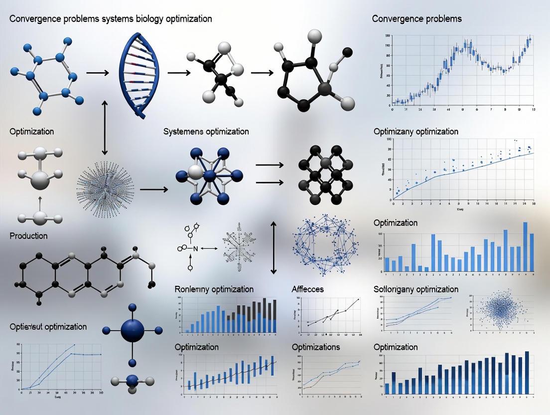
Navigating Convergence Problems in Systems Biology Optimization: From Foundational Challenges to Advanced Solutions

Abstract

This article provides a comprehensive examination of convergence problems encountered in optimization for computational systems biology. Aimed at researchers, scientists, and drug development professionals, it explores the fundamental nature of these challenges in complex biological models, reviews the spectrum of optimization algorithms from deterministic to heuristic methods, presents advanced troubleshooting and hybrid strategies to overcome local optima and stagnation, and establishes rigorous frameworks for methodological validation and comparative performance analysis. By synthesizing insights across these four intents, the article serves as a practical guide for achieving robust, reliable, and biologically meaningful optimization outcomes in biomedical research.

Understanding the Roots: Why Convergence Problems Plague Biological Models

Frequently Asked Questions (FAQs)

Q1: What are the common types of convergence failure in biological optimization? In biological optimization, common convergence failures include:

• Premature Convergence: The algorithm converges to a local optimum, rather than the global optimum, before adequately exploring the parameter space. This is often due to a loss of valuable genetic material in population-based methods [1].
• Stagnation: The optimization progress halts, making no further improvement toward a solution. This can occur in complex problems where the algorithm fails to discover new, better genetic material [1].
• Convergence to a Non-Optimal Structure: The optimization completes but converges to a solution that is not optimal, indicated by a significant energy difference from the true minimum [2].

Q2: My parameter estimation for a differential equation model will not converge. What should I check first? First, investigate your starting values. Convergence can only be expected with fully identified parameters, adequate data, and starting values sufficiently close to the solution estimates [3]. If the estimation fails with default starting values, examine the model and data, then re-run with reasonable, plausible initial guesses [3].

Q3: How can I make my optimization process more robust to initial conditions and avoid local optima?

• Use Global Optimization Methods: Employ multi-start strategies [4], Markov Chain Monte Carlo (MCMC) methods [4], or Genetic Algorithms [4] [5] which are better at exploring the entire parameter space.
• Leverage Uncertainty: Machine learning techniques that quantify prediction uncertainty, such as Gaussian processes, can help algorithms gracefully handle novel data and improve robustness [6].
• Implement a Hierarchical Framework: Models like the Hierarchical Fair Competition (HFC) framework maintain populations of individuals at different fitness levels, providing a continuous supply of new genetic material to prevent premature convergence [1].

Q4: What should I do if my geometry optimization oscillates or the energy does not decrease monotonically? If the energy oscillates around a value and the energy gradient hardly changes, the issue often lies in the calculation setup [7]. To address this:

• Increase Calculation Accuracy: Use a higher numerical quality setting and tighten the SCF convergence criteria [7].
• Check for Electronic Structure Issues: Examine the HOMO-LUMO gap. If it is small and comparable to changes in MO energies between steps, it may cause non-convergence. Verify you have the correct electronic ground state [7].
• Change Optimization Coordinates: Switch from Cartesian to delocalized internal coordinates, which often require fewer steps to converge [7].

Troubleshooting Guides

Guide 1: Resolving SCF Convergence Failures in Quantum Calculations

This guide addresses common Self-Consistent Field (SCF) convergence problems, frequently encountered in electronic structure calculations relevant to biological systems [2].

• Step 1: Analyze the Output Check the end of your output file for error messages. A successful calculation will show a "Job completed" message, while failures may note a large density change or exceeding the maximum number of iterations [2].

• Step 2: Restart the Calculation with Modifications Use the automatically generated restart file (e.g., job_name.01.in). Remove the first MAEFILE line and add igonly=0 to the &gen section to force the SCF to run [2].

• Step 3: Apply Specific Solutions The table below summarizes common fixes and when to apply them [2].

Remedy	Keyword / Action	When to Use
Use a Smaller Basis Set	basis= (e.g., switch to 6-31G)	Primary recommendation for most cases. Start small and gradually increase basis set size [2].
Decrease Accuracy Cutoff	iacc=3	If convergence is sub-optimal with standard settings [2].
Increase Maximum Iterations	maxitg>100	If the system is near convergence when the iteration limit is reached [2].
Enable Failsafe Mode	nofail=1	Lets Jaguar employ special measures automatically when poor convergence is detected [2].
Remove Pseudospectral Grid	nops=1	A more obscure option if other methods fail [2].

Guide 2: Addressing General Optimization Non-Convergence

This guide provides a general workflow for troubleshooting optimization failures in computational biology.

• Step 1: Verify the Problem Setup

  • Check Bounds: Ensure all tuned parameters have appropriate minimum and maximum values. An overly restricted search region can prevent convergence [8].
  • Simplify the Problem: Reduce the number of tuned parameters. Remove parameters that only mildly influence the response, optimize the key parameters, then add the others back [8].
  • Review Constraints: Ensure your constraints and design requirements are achievable. Overly tight specifications can make a feasible solution impossible [8].

• Step 2: Adjust the Optimization Strategy

  • Use a Search-Based Method First: For problems with local minima, run a global search method (e.g., pattern search) to get closer to an acceptable solution before using a gradient-based method [8].
  • Restart from a Different Point: If the optimization converges to an unacceptable local minimum, restart the process from a different initial guess [8].
  • Increase Convergence Tolerances: If the optimization is slow, increasing tolerances can force earlier termination when the solution is "good enough" [8].

• Step 3: Leverage Advanced and Robust Frameworks For persistent issues with complex, multi-parameter models, consider advanced strategies:

  • Optimal Experimental Design (OED): Use mathematical techniques to design experiments that provide maximally informative data for parameter inference, reducing uncertainty and aiding convergence [9] [10].
  • Reinforcement Learning (RL): Apply RL agents, which can be trained over a distribution of parameters, to create robust experimental controllers that are less sensitive to initial parametric uncertainty [10].

Experimental Protocols

Protocol 1: Parameter Estimation for a Non-Linear Biological Model using Multi-Start

This protocol uses a multi-start non-linear least squares (ms-nlLSQ) approach to fit parameters of a model, such as the Lotka-Volterra system [4].

1. Problem Formulation: Define the objective function. For the Lotka-Volterra model (Prey: y, Predator: z), the cost function c(θ) could be the sum of squared differences between simulated and experimental population data, with parameter vector θ = (α, a, b, β) [4].

2. Optimization Execution:

• Generate Starting Points: Create a large set (e.g., 1000) of initial parameter guesses θ₀, randomly sampled from a physiologically plausible range.
• Run Local Optimizations: For each starting point, run a local non-linear least squares optimizer (e.g., Gauss-Newton).
• Collect Results: Gather all final parameter sets and their corresponding cost function values.

3. Solution Analysis:

• Cluster the results to identify local minima.
• Select the parameter set with the lowest objective value as the global solution.

Protocol 2: Biomarker Identification using a Simple Genetic Algorithm (sGA)

This protocol outlines a heuristic method for identifying a minimal set of features (biomarker) for sample classification [4].

1. Problem Encoding:

• Represent a potential biomarker (a set of features) as an individual in a population.
• Encode the individual as a binary string (chromosome) where each bit indicates the presence (1) or absence (0) of a specific feature.

2. Algorithm Execution:

• Initialization: Generate an initial population of random binary strings.
• Evaluation: Calculate the fitness of each individual using a cost function c(θ), which could be a combination of classification accuracy and the number of selected features (to promote a short list).
• Selection, Crossover, Mutation: Create a new generation by:
  • Selection: Choosing parents with a probability proportional to their fitness.
  • Crossover: Combining parts of the parents' chromosomes to produce offspring.
  • Mutation: Randomly flipping bits in the offspring's chromosome with a low probability to introduce new genetic material [4] [5].
• Termination: Repeat the evaluation-selection-mutation cycle for a fixed number of generations or until convergence.

Visualizing Convergence Failure and Solutions

Diagram 1: Optimization Convergence Failure Pathways

This diagram illustrates common failure pathways in optimization algorithms and general strategies to overcome them.

Diagram 2: SCF Convergence Troubleshooting Workflow

This diagram provides a step-by-step decision tree for resolving SCF convergence failures in quantum chemistry calculations [2].

The Scientist's Toolkit: Research Reagent Solutions

The table below lists key computational tools and their functions for addressing convergence problems in systems biology optimization.

Tool / Reagent	Function in Convergence Analysis
Multi-Start Algorithms [4]	A deterministic global optimization strategy that runs local searches from multiple starting points to find the global minimum.
Markov Chain Monte Carlo (MCMC) [4]	A stochastic method for fitting models, particularly useful when the model involves stochastic equations or simulations.
Genetic Algorithms (GA) [4] [5]	A population-based, heuristic method inspired by natural selection, effective for a broad range of optimization problems, including model tuning and biomarker identification.
Hierarchical Fair Competition (HFC) [1]	An evolutionary framework that prevents premature convergence by maintaining subpopulations at different fitness levels and enabling continuous discovery of new genetic material.
Reinforcement Learning (RL) [10]	An AI method that learns optimal experimental designs (policies) through trial and error, offering robustness to parametric uncertainty.
Fisher Information Matrix [10]	A mathematical construct used in Optimal Experimental Design (OED) to maximize the informativeness of experiments for parameter estimation.
Roxatidine	Roxatidine, CAS:78273-80-0, MF:C17H26N2O3, MW:306.4 g/mol
Farnesyl acetate	Farnesyl acetate, CAS:29548-30-9, MF:C17H28O2, MW:264.4 g/mol

Frequently Asked Questions (FAQs)

Q1: Why does my systems biology model fail to converge to a solution during optimization? A1: Convergence problems often stem from the inherent high-dimensionality and non-linearity of biological systems. As model complexity increases with more parameters and reactions, the parameter space expands exponentially, making it difficult for optimization algorithms to find a global optimum. This is compounded by non-linear dynamics that create complex, multi-modal fitness landscapes where algorithms can become trapped in local minima [11] [12].

Q2: What is the difference between local and global sensitivity analysis, and why does it matter for convergence? A2: Local sensitivity analysis (e.g., one-at-a-time parameter variation) assesses parameter importance at a single operating point in parameter space, making it computationally efficient but unreliable for non-linear models where parameter influences change across different regions. Global sensitivity analysis (e.g., PRCC, eFAST) varies all parameters simultaneously over wide ranges, quantifying their influence and interactions across the entire parameter space. For complex models, relying solely on local sensitivity can misguide optimization by overlooking critical parameter interactions, leading to convergence failure on suboptimal solutions [11] [12].

Q3: How can I manage the computational cost of global sensitivity analysis for my high-dimensional model? A3: Employing surrogate models (emulators) is a key strategy. A surrogate model is a machine learning model (e.g., neural network, random forest, Gaussian process) trained on a subset of simulation data to predict model outputs for new parameter sets. This replaces computationally expensive simulations, drastically reducing the time required for sensitivity analysis and optimization. This approach has been shown to replicate sensitivity analysis results while reducing processing time from hours to minutes [12].

Q4: My multi-omics data integration is not yielding biologically meaningful clusters. What could be wrong? A4: This issue often arises from incorrect weighting or misalignment of different data modalities. Ensure that preprocessing and normalization are appropriate for each data type (e.g., RNA-seq, ATAC-seq). Utilizing frameworks like MUON, which are designed for multimodal data, can help. These frameworks allow for applying modality-specific processing and then integrating them using methods like Multi-Omic Factor Analysis (MOFA) or Weighted Nearest Neighbors (WNN) to create a balanced joint representation for clustering [13].

Q5: Which optimization algorithm should I choose for my biological model? A5: The choice depends on your model's characteristics. The table below summarizes common options:

Table: Comparison of Optimization Algorithms for Biological Systems

Algorithm	Principle	Best For	Strengths	Weaknesses
Genetic Algorithm (GA) [5]	Natural selection, crossover, mutation	Complex, multi-modal problems; global optimization	Robust, good global search, avoids local minima	Computationally expensive, parameter tuning
Particle Swarm Optimization (PSO) [11] [5]	Social behavior of bird flocking/fish schooling	Continuous optimization problems	Simple, computationally efficient, fast convergence	Can converge prematurely to local minima
Grey Wolf Optimizer (GWO) [5]	Social hierarchy and hunting behavior of grey wolves	Exploration/exploitation balance	Simple, few parameters to tune, strong performance	May struggle with very high-dimensional problems

Troubleshooting Guides

Issue: Optimization Fails to Converge or Converges to Physiologically Implausible Solutions

Diagnosis Steps:

• Check Parameter Identifiability: Determine if your experimental data is sufficient to uniquely estimate all model parameters. An unidentifiable model has multiple parameter sets yielding identical fits, preventing convergence to a unique solution.
• Perform a Global Sensitivity Analysis (GSA): Use GSA to identify which parameters most strongly influence your model output. This reveals the core set of parameters that the optimization must focus on.
• Profile the Objective Function: Visualize the objective function (e.g., cost landscape) with respect to key sensitive parameters. A rugged landscape with many local minima indicates a challenging optimization problem.

Resolution Protocols:

• Protocol 1: Implement Robust Sampling. Use Latin Hypercube Sampling (LHS) instead of simple random sampling for GSA. LHS ensures better stratification and coverage of the high-dimensional parameter space with fewer samples, leading to more reliable sensitivity indices [12].
• Protocol 2: Apply a Hybrid Optimization Strategy. Combine a global optimizer (e.g., Genetic Algorithm) to broadly explore the parameter space and avoid local minima, with a local optimizer (e.g., gradient-based method) to refine the solution and achieve fast final convergence.
• Protocol 3: Utilize Surrogate-Assisted Optimization. For computationally intensive models, train a surrogate model to approximate the simulation output. Perform the majority of optimization iterations on the fast surrogate, only using the full model for final validation [12].

Issue: Poor Performance in Multi-Modal Data Integration and Cross-Modal Prediction

Diagnosis Steps:

• Assess Modality Quality Individually: First, analyze each data modality (e.g., transcriptomics, proteomics) separately using established single-omics workflows to ensure each dataset is of high quality and contains meaningful biological signal.
• Check for Batch Effects: Determine if technical artifacts are causing cells/samples to cluster by batch rather than biological identity within each modality.
• Evaluate Integration Metrics: Use quantitative metrics to assess integration performance, such as the mixing of biologically similar cell types across batches and the conservation of cell-type-specific features.

Resolution Protocols:

• Protocol 1: Employ a Multi-Task Learning Framework. Use a framework like UnitedNet, which alternates training between joint group identification (e.g., clustering) and cross-modal prediction tasks. This has been shown to improve performance in both tasks by reinforcing learning through a shared latent space [14].
• Protocol 2: Leverage Specialized Multi-Modal Frameworks. Adopt a data structure and analysis framework like MUON, which is specifically designed for multimodal omics. It allows for modality-specific preprocessing and provides interfaces to multiple integration methods (MOFA, WNN) for flexible and efficient analysis [13].
• Protocol 3: Incorporate Explainable AI (XAI). Dissect a trained multi-modal model with XAI algorithms like SHAP (SHapley Additive exPlanations). This can quantify cell-type-specific, cross-modal feature relationships (e.g., which DNA accessibility peaks are most relevant to a gene's expression in a specific cell type), providing biological validation and insights [14].

Experimental Protocols

Protocol: Global Sensitivity Analysis for a Multi-Scale Model Using Variance-Based Methods

Objective: To quantify the contribution of each input parameter to the variance of the output in a complex, non-linear multi-scale model, identifying key drivers and potential candidates for model reduction.

Materials & Computational Tools:

• Software: COPASI [11], MUON (for multi-omics) [13], or custom scripts in Python/R.
• Sampling Method: Latin Hypercube Sampling (LHS) [12].
• Sensitivity Method: Extended Fourier Amplitude Sensitivity Test (eFAST) or Sobol method [12].

Step-by-Step Methodology:

• Parameter Selection and Ranging: Define the list of N parameters for analysis. Set a biologically plausible range for each parameter (e.g., ±2 orders of magnitude from a nominal value). Log-transform parameters if ranges span multiple orders of magnitude.
• Generate Parameter Sets: Use LHS to generate K parameter sets from the defined N-dimensional space. The number of sets K should be at least an order of magnitude larger than N [12].
• Model Execution: Run the model simulation for each of the K parameter sets and record the output(s) of interest (e.g., steady-state concentration, oscillation amplitude).
• Calculate Sensitivity Indices: For a chosen output, apply the eFAST or Sobol method to compute:
  • First-Order (Main) Index (Si): Measures the fractional contribution of each parameter alone to the output variance.
  • Total-Order Index (STi): Measures the total contribution of each parameter, including all interaction effects with other parameters.
• Statistical Inference: Use a dummy parameter (a parameter known to have no effect) to establish a significance threshold. Sensitivity indices above this threshold are considered meaningful.
• Interpretation: Parameters with high STi values are the most influential and should be prioritized for accurate estimation. Parameters with very low STi may be fixed to constant values for model reduction.

Table: Key Reagents and Computational Tools for GSA

Item Name	Function/Brief Explanation	Example/Note
COPASI	Software for simulation and analysis of biochemical networks	Used for optimization and Metabolic Control Analysis [11]
Latin Hypercube Sampling (LHS)	A stratified sampling technique for efficient exploration of parameter space	Ensures full coverage of each parameter's range [12]
eFAST/Sobol Method	Variance-based global sensitivity analysis methods	Quantifies main and total-order effect indices [12]
Surrogate Model (Emulator)	A machine learning model trained to approximate a complex simulation	Neural Networks, Gaussian Processes; reduces computational cost [12]

Workflow Diagram: Global Sensitivity and Optimization Pipeline

Protocol: Multi-Modal Data Integration with UnitedNet

Objective: To integrate multiple data modalities (e.g., gene expression and chromatin accessibility) for joint cell-type identification and cross-modal prediction, while enabling the discovery of cell-type-specific feature relationships.

Materials & Computational Tools:

• Framework: UnitedNet [14] or MUON [13].
• Data: A multi-modal single-cell dataset (e.g., multiome ATAC+Gene Expression, CITE-seq).

Step-by-Step Methodology:

• Data Preprocessing: Independently preprocess each modality using standard workflows (quality control, normalization, feature selection) for RNA-seq, ATAC-seq, etc.
• Model Configuration: Set up the UnitedNet architecture with:
  • Modality-specific encoders to generate latent codes from each data type.
  • A fusion module to combine codes into a shared latent representation.
  • Task-specific decoders/classifiers for joint clustering and cross-modal prediction.
  • Discriminators (adversarial) to improve prediction realism.
• Multi-Task Training: Train the network by alternating between:
  • Task A (Joint Group Identification): Minimizing a combined loss of clustering/classification loss and a contrastive loss to align modalities.
  • Task B (Cross-Modal Prediction): Minimizing a combined loss of prediction error and an adversarial (generator) loss.
• Model Explanation: Apply the SHAP explainable AI algorithm to the trained UnitedNet. This quantifies the contribution of features from one modality (e.g., accessibility of a genomic peak) to the prediction of features in another modality (e.g., expression of a gene) for specific cell types.
• Biological Validation: The SHAP-derived, cell-type-specific feature relationships represent hypotheses about gene regulation (e.g., enhancer-promoter interactions) that can be validated with orthogonal experimental techniques.

Workflow Diagram: Multi-Modal Integration with UnitedNet

Inverse Problems and Ill-Posed Formulations in Parameter Estimation for Dynamic Models

Troubleshooting Guides

Guide: Addressing Convergence Failures in Dynamic Model Calibration

Reported Issue: The parameter estimation algorithm fails to converge to a plausible solution, or results vary dramatically with different initial guesses.

Explanation: Convergence failures in dynamic models of biological systems often stem from two fundamental pathological characteristics of the inverse problem: ill-conditioning and nonconvexity [15]. Ill-conditioning arises from over-parametrization, experimental data scarcity, and significant measurement errors. Nonconvexity leads to multiple local minima in the objective function, causing algorithms to converge to suboptimal solutions that are estimation artefacts rather than true biological parameters [15].

Resolution Steps:

• Diagnose Ill-Conditioning:

  • Check parameter correlation matrices for values near ±1.0, indicating unidentifiable parameters.
  • Examine the eigenvalues of the Hessian (or Fisher Information) matrix; large condition numbers (ratio of largest to smallest eigenvalue) confirm ill-conditioning.
  • Perform a posteriori identifiability analysis (e.g., via profile likelihood) to pinpoint non-identifiable parameters.

• Implement Regularization to Combat Ill-Conditioning:

  • Introduce a regularization term to your objective function. This penalizes overly complex solutions and reduces overfitting.
  • Tikhonov Regularization: Adds a penalty proportional to the squared deviation of parameters from a prior guess, biasing solutions toward simpler, more stable values.
  • Properly tune the regularization parameter to achieve the best trade-off between bias and variance, ensuring the model generalizes well to new data [15].

• Address Nonconvexity with Global Optimization:

  • Replace local optimization methods (e.g., lsqnonlin) with efficient global optimization (EGO) methods.
  • Use multi-start strategies with a large number of starts (hundreds to thousands) from random initial points within physiologically plausible parameter bounds.
  • This minimizes the possibility of convergence to local solutions and helps locate the global minimum [15].

Guide: Mitigating Overfitting and Poor Predictive Performance

Reported Issue: The calibrated model fits the training data well but performs poorly on validation data, indicating low predictive value and overfitting.

Explanation: Overfitting occurs when a model learns the noise in the calibration data instead of the underlying biological signal. This is common in systems biology due to model over-parametrization and information-poor data. Overfitting damages the model's predictive and explanatory power [15].

Resolution Steps:

• Simplify the Model Structure:

  • Use the simplest model structure that adequately captures system dynamics. AR and ARX model structures are good first candidates due to simpler, more robust estimation algorithms [16].
  • Check the model order. An order that is too low (under-fitting) prevents a good fit, while an order that is too high (over-fitting) makes parameters highly sensitive to noise [16].

• Apply Regularization Techniques:

  • As in Guide 1.1, use regularization to penalize model complexity explicitly. This is a systematic way to incorporate prior knowledge and prevent the model from fitting the noise [15].

• Improve Data Quality and Information Content:

  • Ensure inputs adequately excite the system dynamics. Simple inputs like step changes are often insufficient; inject extra input perturbations [16].
  • Preprocess data to handle deficiencies like drift, offset, missing samples, and outliers [16].
  • If possible, employ optimal experimental design (OED) to design experiments that maximize information gain for parameter estimation.

Logical Relationship of Parameter Estimation Challenges and Solutions

Frequently Asked Questions (FAQs)

Model Structure and Initialization

Q1: What is the simplest model structure to start with for linear dynamic systems to avoid estimation difficulties?

A: For time-series models (no inputs), begin with an AutoRegressive (AR) structure. For input-output models, start with an AutoRegressive with eXogenous inputs (ARX) structure. The estimation algorithms for AR and ARX are simpler and less sensitive to initial parameter guesses than more complex structures like ARMA or ARMAX [16]. For systems linear in parameters but not fitting AR/ARX forms, Recursive Least Squares (RLS) estimation is a robust alternative that can handle some nonlinearities [16].

Q2: How critical are initial parameter guesses, and how should I set them?

A: Specifying initial parameter guesses and their initial covariance is highly recommended [16]. The initial guess should be based on prior knowledge of the system or from offline estimation. The initial covariance represents your uncertainty in the guess. If you are confident in your initial values, specify a smaller initial parameter covariance; the default value of 10000 is often too large, causing the estimator to initially ignore your guess [16]. This is especially important for complex model structures (ARMA, ARMAX, etc.) to avoid the algorithm finding a poor local minima [16].

Data and Algorithm Configuration

Q3: My estimation data is from a simple step experiment. Why does the estimation perform poorly?

A: Simple inputs like a step often do not provide sufficient excitation for estimating more than a very limited number of parameters [16]. They may fail to activate all the relevant system dynamics. The solution is to design input signals that better perturb the system, such as pseudo-random binary sequences (PRBS) or chirp signals, or to inject extra input perturbations during operation [16].

Q4: For a forgetting factor algorithm, how do I choose the right forgetting factor (λ)?

A: The forgetting factor, λ, controls the algorithm's memory. If λ is too small (closer to 0), the algorithm assumes parameters vary quickly with time, making it agile but also noisy. If λ is too large (closer to 1), the algorithm assumes parameters are nearly constant, leading to slow adaptation to real changes. Choose λ based on the expected rate of parameter change in your specific system [16].

Advanced Challenges and Solutions

Q5: What are the root causes of overfitting in dynamic biological models, and how is it systematically addressed?

A: The root causes are ill-conditioning (from over-parametrization and data scarcity) and excessive model flexibility [15]. This causes the model to fit the calibration data's noise, harming its predictive value. The systematic solution involves regularization, which adds a penalty term to the objective function to constrain parameter values. This ensures the best trade-off between bias and variance, effectively reducing overfitting and allowing for the incorporation of prior knowledge in a principled way [15].

Q6: Why are local optimization methods often insufficient for parameter estimation in nonlinear dynamic models?

A: The parameter estimation problem for these models is often nonconvex and multi-modal, meaning the cost function landscape has multiple local minima [15]. Standard local methods can easily get stuck in one of these local solutions, which may be far from the global optimum, leading to incorrect conclusions about the model's validity or the system's biology. Therefore, global optimization methods are generally required to robustly find the best fit [15].

The Scientist's Toolkit: Research Reagent Solutions

Table 1: Key Computational Tools and Methods for Robust Parameter Estimation.

Item/Reagent	Function/Benefit	Application Note
AR/ARX Model Structures	Simpler, more robust estimation algorithms; good first candidates for linear systems [16].	Use AR for time-series; ARX for input-output models. Less sensitive to initial guesses.
Efficient Global Optimization (EGO)	Addresses nonconvexity; minimizes convergence to local minima by searching parameter space globally [15].	Preferred over multi-start local methods for complex, rugged cost function landscapes.
Tikhonov Regularization	Combats ill-conditioning & overfitting by adding a constraint to the objective function, biasing solutions toward stability [15].	Essential for over-parametrized models. Requires careful tuning of the regularization parameter.
Recursive Least Squares (RLS)	A versatile estimation algorithm for models linear in their parameters, capable of handling some nonlinearities [16].	More flexible than ARX; useful when the model does not fit a standard polynomial form.
Profile Likelihood Analysis	A posteriori analysis method for diagnosing practical parameter identifiability [15].	Identifies which parameters can be uniquely estimated from the available data.
Cannflavin B	Cannflavin B, CAS:76735-58-5, MF:C21H20O6, MW:368.4 g/mol	Chemical Reagent
Norchelerythrine	Norchelerythrine

Workflow for Robust Parameter Estimation

Computational Complexity and the NP-Hard Nature of Global Optimization in Pathway Analysis

Frequently Asked Questions

What does it mean that global optimization in PEA is NP-hard? In computational complexity theory, an NP-hard problem is at least as difficult as the hardest problems in the class NP. Finding a polynomial-time algorithm for any NP-hard problem would solve all problems in NP in polynomial time, which is suspected to be impossible (P ≠ NP hypothesis) [17]. Global optimization in Pathway Enrichment Analysis (PEA), which involves searching through vast combinatorial spaces of gene interactions and pathway topologies to find the optimally enriched set, often falls into this category. This means that as the size of your input (e.g., the number of genes or the complexity of the pathway network) grows, the computational time required to find the guaranteed best solution can grow exponentially, making exact optimization intractable for large datasets [17].

Why does the NP-hard nature of the problem lead to convergence issues in my analysis? Because most PEA software relies on heuristic or metaheuristic algorithms (e.g., Genetic Algorithms, Particle Swarm Optimization) to find good, but not necessarily perfect, solutions in a reasonable time [5]. These algorithms may converge to a local optimum—a solution that is better than its immediate neighbors but not the best overall solution in the entire search space. When an analysis converges to a local optimum, you might get a plausible-looking list of enriched pathways that is not biologically representative, leading to misinterpretations.

My enrichment analysis produced different results using the same gene list on two different tools. Is this related to optimization? Yes, this is a common manifestation of the underlying computational challenge. Different PEA tools employ different algorithms and heuristics to navigate the NP-hard solution space [18]. For example:

• g:Profiler g:GOSt primarily uses a modified Fisher's exact test for over-representation analysis (ORA) [18].
• GSEA uses a method that considers the ranking of genes and is a mix of self-contained and competitive methods [18].
• Topology-based PEA (TPEA) tools incorporate network topology, which adds another layer of complexity [18]. Each algorithm has a different search trajectory and may therefore converge on a different subset of "top" pathways from the vast possibilities.

How can I improve confidence in my results given these convergence problems?

• Use Multiple Tools: Run your analysis using several different methods (e.g., both ORA and GSEA) and compare the results. Pathways that are consistently enriched across multiple algorithms are more robust [18].
• Benchmark Your Input: Adhere to the principle of "garbage in, garbage out." Ensure the quality of your input gene list, as poor-quality input will exacerbate convergence issues and produce misleading outputs [18].
• Leverage Topology: When possible, use topology-based methods, as they can provide more precise results by accounting for gene interactions, though they are computationally more intensive [18].

Troubleshooting Guide

Problem: Analysis fails to complete or times out. This often occurs with large input gene lists or complex pathway databases where the search space becomes prohibitively large.

• Solution 1: Filter your input gene list to a more focused set (e.g., using a stricter p-value or fold-change cutoff) to reduce problem size [18].
• Solution 2: Check the computational resources. For large analyses, ensure you are using a system with sufficient memory and processing power, or switch to a tool designed for high-performance computing.
• Solution 3: Simplify the analysis. Start with a more common ORA before moving to a more complex topology-based PEA.

Problem: Results are inconsistent between repeated runs. Some optimization algorithms, like Genetic Algorithms, have a stochastic (random) component. If your tool uses such methods, results can vary between runs.

• Solution 1: Increase the number of iterations or generations in the algorithm's settings. This gives the algorithm more time to stabilize.
• Solution 2: Use a fixed random seed if the tool allows it. This ensures the "random" process is the same each time, leading to reproducible results.
• Solution 3: As a best practice, always run stochastic algorithms multiple times and aggregate the results (e.g., report pathways that appear in a majority of runs).

Problem: Results do not match biological expectations. The algorithm may have converged to a mathematically local but biologically irrelevant optimum.

• Solution 1: Manually curate the background gene set or the pathway database to better reflect your experimental context (e.g., tissue-specific pathway databases) [18].
• Solution 2: Adjust the algorithm's parameters. For instance, in a Genetic Algorithm, increasing the mutation rate can help the search "jump" out of local optima [5].
• Solution 3: Clearly define your analysis type (ORA, GSEA, TPEA) and data type (unordered list, ranked list, expression data) before starting, as using an inappropriate method is a common source of error [18].

Experimental Protocols for Cited Key Experiments

Protocol 1: Benchmarking Heuristic Performance in PEA

This protocol assesses the performance of different optimization algorithms on a standard PEA task.

• Data Preparation: Obtain a canonical gene list with a known, well-established pathway association (a "gold standard" dataset) from published literature.
• Tool Selection: Select several PEA tools that use different optimization strategies (e.g., one using a deterministic method like Fisher's exact test, one using a Genetic Algorithm (GA), and one using Particle Swarm Optimization (PSO)) [18] [5].
• Parameter Configuration: For heuristic-based tools (GA, PSO), set a low iteration count (e.g., 100 generations) to simulate premature convergence. Use a high iteration count (e.g., 1000 generations) for a positive control.
• Execution: Run all tools on the gold standard dataset using both low and high iteration settings.
• Evaluation: Compare the output enriched pathways against the known gold standard pathway. Metrics to track are shown in the table below.

Table 1: Metrics for Benchmarking Heuristic Performance

Metric	Description	How to Measure
Recall	The ability to identify the known true pathway.	(Number of tools that found the gold standard pathway) / (Total number of tools run)
Runtime	Computational time required.	Record wall-clock time for each tool/run.
Convergence Iteration	The point where the solution stabilizes.	For heuristic tools, plot the fitness score over iterations (see Diagram 1).
Result Stability	Consistency of results across multiple runs.	Run stochastic algorithms 10 times and calculate the Jaccard index of the top 10 pathways between runs.

Protocol 2: Comparing ORA vs. GSEA on a Ranked Gene List

This protocol highlights how the choice of method, driven by the nature of the optimization problem, affects outcomes.

• Data Preparation: Start with a ranked list of genes (e.g., from a differential expression analysis).
• Tool Execution: Input the same ranked list into two analyses:
  • ORA: Use a tool like g:Profiler g:GOSt in its ORA mode, which requires applying a strict cutoff (e.g., top 100 genes) to create a non-ranked list [18].
  • GSEA: Use a tool like the Broad Institute's GSEA software, which uses the entire ranked list without a cutoff [18].
• Analysis: Compare the top 10 enriched pathways from each method. Note that ORA will highlight pathways overrepresented in your top 100 genes, while GSEA will highlight pathways whose genes are concentrated at the extreme ends (top or bottom) of your entire ranked list.

Optimization Convergence Workflow

The following diagram illustrates the typical workflow and decision points when dealing with convergence problems in PEA optimization.

The Scientist's Toolkit: Research Reagent Solutions

Table 2: Essential Tools and Databases for Pathway Enrichment Analysis

Item Name	Type	Primary Function
g:Profiler g:GOSt [18]	Web Tool / Software	Performs functional enrichment analysis (ORA) on unordered or ranked gene lists, using multiple testing corrections.
Enrichr [18]	Web Tool	A gene set enrichment analysis web resource that provides various visualization options for results.
GSEA Software [18]	Desktop Application	Implements the Gene Set Enrichment Analysis (GSEA) method, which focuses on ranked gene lists without requiring a strict cutoff.
Ingenuity Pathway Analysis (IPA) [19]	Commercial Software	A comprehensive platform for pathway analysis that integrates data from various 'omics' experiments and uses a curated knowledge base.
KEGG [18]	Pathway Database	A collection of manually drawn pathway maps representing current knowledge on molecular interaction and reaction networks.
Reactome [18]	Pathway Database	An open-source, open-access, manually curated and peer-reviewed pathway database.
Gene Ontology (GO) [18]	Knowledge Base	Provides a structured, controlled vocabulary (ontologies) for describing gene product attributes across species.
Genetic Algorithm (GA) [5]	Optimization Method	A metaheuristic inspired by natural selection used to find approximate solutions to NP-hard optimization problems.
Particle Swarm Optimization (PSO) [5]	Optimization Method	A computational method that optimizes a problem by iteratively trying to improve a candidate solution with regard to a given measure of quality.
Cepharadione B	Cepharadione B|CAS 55610-02-1|Alkaloid
Ferensimycin B	Ferensimycin B, CAS:83852-60-2, MF:C35H62O10, MW:642.9 g/mol	Chemical Reagent

The Impact of Noisy, Sparse, and High-Throughput Experimental Data on Optimization Stability

Troubleshooting Guide: Resolving Convergence Failures

This guide addresses common optimization convergence problems stemming from noisy, sparse, and high-throughput data in systems biology.

Table 1: Troubleshooting Convergence Issues in Optimization

Problem Symptom	Potential Root Cause	Diagnostic Steps	Recommended Solutions
Parameter estimates vary wildly between runs	High sensitivity to experimental noise in the data [20].	Assess signal-to-noise ratio (SNR) in replicate measurements.	Implement sparse regularization to enforce simpler, more robust models [21]; Use trust-region methods like NOSTRA to focus sampling [22].
Algorithm fails to find a good fit even with plausible parameters	Data sparsity insufficient to capture underlying system dynamics [22] [23].	Check if data is "non-space-filling" in the parameter space.	Integrate physics-based constraints (e.g., divergence-free fields) during interpolation [24]; Use cubic splines for very sparse 1D signals [23].
Model converges to different local minima on different datasets	Combination of data noise and sparsity leading to an ill-posed problem [20] [4].	Perform multi-start optimization from different initial points.	Employ global optimization strategies like Genetic Algorithms (GAs) or Markov Chain Monte Carlo (MCMC) [4].
Performance degrades with high-dimensional omics data	Curse of dimensionality; sparse data in high-dimensional space reduces surrogate model accuracy [22].	Analyze surrogate model accuracy (e.g., Gaussian Process cross-validation error).	Apply dimensionality reduction techniques before optimization [22]; Use feature selection to identify a minimal biomarker set [4].
Introduces spurious relationships in inferred networks	Failure to account for latent confounding factors and correlated noise in high-throughput data [25].	Check for strong, unmodeled batch effects in the data.	Use methods like SVA (Surrogate Variable Analysis) to estimate and adjust for latent factors [25].

Frequently Asked Questions (FAQs)

Q1: My data is both very sparse and very noisy. Which issue should I tackle first? Prioritize handling noise first. Noisy data can lead to fundamentally incorrect and biased models, and many interpolation methods (like splines) that work for sparse data are highly sensitive to noise [23] [20]. A robust approach is to use a framework like NOSTRA, which is explicitly designed to handle both challenges simultaneously by integrating prior knowledge of uncertainty and focusing sampling in promising regions [22].

Q2: For high-throughput biological data, what is the most critical step in experimental design to ensure optimization stability? The most critical step is planning for batch effects and biological replication from the outset. Confounding from unmeasured latent factors is a major source of bias that cannot be averaged out [25]. As stated in Modern Statistics for Modern Biology, "To consult the statistician after an experiment is finished is often merely to ask him to conduct a post mortem examination. He can perhaps say what the experiment died of" [25]. You should also start data analysis as soon as the first batch is collected ("dailies") to track unexpected variation early [25].

Q3: When identifying a sparse dynamical model from data, why does noise cause such significant problems? Noise severely impacts the calculation of derivatives, which is a fundamental step in identifying the governing equations [20]. Furthermore, with noise, the measurement data matrix can violate mathematical properties (like the restricted isometry property), making it impossible for standard sparse regression algorithms to correctly identify the underlying model structure [20].

Q4: In the context of antibody discovery, how is high-throughput data generation used to overcome noise and sparsity challenges? The field uses an iterative cycle of high-throughput experimentation and machine learning. Technologies like next-generation sequencing (NGS) and yeast display generate massive datasets on antibody sequences and binding properties [26]. This volume of data helps overcome sparsity, while machine learning models trained on this data can then predict and optimize antibody properties (like affinity and stability), reducing reliance on noisy individual assays and guiding further experiments efficiently [26].

Experimental Protocols for Robust Optimization

Protocol: Model Tuning with Noisy and Sparse Data

This protocol details parameter estimation for a biological model (e.g., a system of ODEs) when experimental data is limited and noisy [4].

• Problem Formulation: Define the optimization problem. The goal is to find the parameter vector (\theta) that minimizes the difference between model simulations and experimental data (y(\bm{x})).

  • Objective Function: Often formulated as a non-linear least squares problem: (c(\theta) = \sum (y(\bm{x}) - \hat{y}(\bm{x}, \theta))^2), where (\hat{y}) is the model output [4].
  • Constraints: Incorporate known biological constraints, such as non-negative rate constants or known parameter relationships [4].

• Surrogate Model Enhancement (for very scarce data): To improve the accuracy of the surrogate model (e.g., Gaussian Process):

  • Integrate prior knowledge of experimental uncertainty directly into the model [22].
  • Use trust regions to dynamically focus computational resources on areas of the parameter space with a high probability of containing optimal solutions [22].

• Optimization Algorithm Selection:

  • Multi-start Non-Linear Least Squares (ms-nlLSQ): A deterministic approach suitable for continuous parameters and objective functions. Run a local optimizer (e.g., Gauss-Newton) from multiple starting points to find the global minimum [4].
  • Genetic Algorithm (sGA): A heuristic, population-based method effective for non-convex problems and those with discrete or continuous parameters. It is less likely to get stuck in local minima [4].
  • Markov Chain Monte Carlo (rw-MCMC): A stochastic method ideal for problems involving stochastic simulations or when a full posterior distribution of parameters is desired [4].

• Validation: Validate the identified parameters on a held-out dataset not used during training. Perform robustness analysis by testing how parameter estimates change with slight perturbations in the input data.

Protocol: Biomarker Identification from High-Throughput Omics Data

This protocol outlines the process of identifying a minimal set of features (e.g., genes, proteins) for classifying samples, a common optimization problem in systems biology [4].

• Data Acquisition and Preprocessing:

  • Acquire high-dimensional data (e.g., RNA-Seq, proteomics) from samples belonging to different classes (e.g., healthy vs. diseased) [27].
  • Preprocess and normalize the data rigorously to account for technical artifacts (e.g., sequencing depth, batch effects) [27] [25].

• Feature Selection as Optimization: Formulate the selection of a biomarker of size (k) as an optimization problem.

  • Parameters ((\theta)): The list of (k) features to select.
  • Objective Function ((c(\theta))): A function that scores the selected features, such as the cross-validated accuracy of a classifier (e.g., a linear discriminant analysis) built using those features [4].

• Algorithm Execution:

  • Apply a Global Optimization algorithm like a Genetic Algorithm (GA) to efficiently search the vast space of possible feature combinations [4].
  • The GA will evolve a population of potential feature sets through selection, crossover, and mutation, favoring sets that yield higher classification accuracy.

• Validation and Final Model Building:

  • Validate the final selected biomarker on an completely independent test set.
  • Use the identified features to build a final, robust classifier for predicting sample categories in new data.

Workflow Visualization

Optimization Stability Workflow

The Scientist's Toolkit: Research Reagent Solutions

Table 2: Key Experimental Technologies for High-Throughput Data Generation

Technology / Reagent	Primary Function	Role in Managing Noise/Sparsity
Next-Generation Sequencing (NGS) [26]	High-throughput sequencing of antibody repertoires or transcriptomes.	Generates massive datasets, overcoming sparsity by providing a deep view of biological diversity.
Yeast Display [26]	Surface expression of antibodies for screening against antigens.	Enables high-throughput functional screening of vast libraries (>10^9 variants), efficiently exploring sequence space.
Bio-Layer Interferometry (BLI) [26]	Label-free quantification of binding kinetics and affinity.	Provides high-quality, quantitative binding data for many samples, improving signal and reducing noise for model training.
Differential Scanning Fluorimetry (DSF) [26]	High-throughput assessment of protein (e.g., antibody) stability.	Allows rapid ranking of stability for hundreds of candidates, adding a critical, low-noise parameter for optimization.
Constrained Cost Minimization (CCM) [24]	A computational interpolation technique for sparse particle tracks.	Incorporates physical constraints (e.g., divergence-free velocity) to denoise and improve data quality from sparse measurements.
Pyrrolomycin D	Pyrrolomycin D, CAS:81910-07-8, MF:C11H4Cl5NO2, MW:359.4 g/mol	Chemical Reagent
Dapabutan	Dapabutan (DAS-01) PPAR α/δ Agonist|RUO

Algorithmic Arsenal: Optimization Methods for Biological Systems

Frequently Asked Questions (FAQs)

FAQ 1: What are the fundamental differences between linear and nonlinear programming?

• Linear Programming (LP) is a mathematical optimization technique where the objective function and all constraints are linear. It is used to find the best outcome (such as maximum profit or lowest cost) in a model whose requirements are represented by linear relationships. Solutions can be found using methods like the simplex method or interior-point methods [28].
• Nonlinear Programming (NLP) deals with optimization problems where the objective function or constraints are nonlinear. This allows for modeling more complex, real-world relationships but introduces challenges like multiple local optima and increased computational difficulty. Solutions often require iterative numeric methods like gradient descent or Newton's method [28] [29].

FAQ 2: Why do deterministic models like LP and NLP often fail in biological systems? Biological systems are inherently "messy," characterized by stochasticity (randomness), low copy numbers of molecules (e.g., genes), and combinatorial complexity. Deterministic models, which produce the same output for a given input without room for random variation, often fail to capture this intrinsic noise and can yield unrealistic results [30]. For instance, a deterministic model might predict a smooth, continuous output for gene expression, whereas experimental data show noisy, burst-like expression [30].

FAQ 3: What are convergence problems in systems biology optimization? In optimization, convergence refers to the algorithm reaching a stable, optimal solution. Problems arise when algorithms:

• Get trapped in local optima instead of the global optimum, which is a common issue in non-convex NLP problems [28].
• Fail to converge within a reasonable time frame due to high-dimensional parameter spaces or complex, ill-behaved objective functions, a frequent challenge when modeling biological networks with many interacting components [31].
• Exhibit oscillatory behavior instead of smoothly approaching an optimum, which can occur with some accelerated gradient methods [32].

FAQ 4: How can I check if my optimization algorithm has converged? For Bayesian optimization, which uses probabilistic surrogate models, one can monitor the Expected Improvement (EI). A framework inspired by Statistical Process Control (SPC) can be used to check for a decrease in EI and the stability of its variance to assess convergence more reliably than using a simple threshold [31]. For traditional LP/NLP, convergence is often declared when changes in the objective function or solution variables between iterations fall below a predefined tolerance.

FAQ 5: When should I use deterministic vs. stochastic approaches in biological modeling?

• Use deterministic models (LP/NLP) when dealing with systems where the statistics of large numbers apply, yielding an average behavior that is a good approximation (e.g., metabolic pathways with abundant metabolites) [30].
• Use stochastic models when the system involves low copy numbers of key components (e.g., gene expression), discrete events, or when heterogeneity and noise are critical to the system's function (e.g., cell fate decisions) [30].

Troubleshooting Guides

Problem 1: Model Infeasibility or Unrealistic Solutions

Symptoms: The solver returns an "infeasible" error, or the solution is biologically impossible (e.g., negative concentrations).

Potential Cause	Diagnostic Steps	Solution Strategies
Overly Restrictive Linear Constraints	Check the feasibility of each constraint against expected biological ranges.	Reformulate constraints; use softer constraints with penalty terms; switch to NLP for more flexible formulation [28].
Oversimplified Model	Compare model predictions with simple experimental data.	Incorporate nonlinear relationships (e.g., Michaelis-Menten kinetics instead of linear rates); add critical missing biological details [30] [33].
Incorrect Bounds on Variables	Review the lower and upper bounds set for all decision variables (e.g., reaction rates).	Adjust variable bounds based on literature or experimental measurements.

Problem 2: Optimization Fails to Converge or Converges Slowly

Symptoms: The solver exceeds the maximum number of iterations, the objective function oscillates, or progress stalls.

Potential Cause	Diagnostic Steps	Solution Strategies
Ill-Conditioned Problem	Check the condition number of the Hessian (for NLP) or the constraint matrix (for LP).	Scale variables and constraints to similar magnitudes; reformulate the problem to improve numerical properties [28].
Trapped in Local Optima	Run the optimization from multiple different initial starting points and compare results.	Use global optimization methods (e.g., genetic algorithms); implement multistart strategies; use algorithms with momentum (e.g., Nesterov acceleration) [28] [32].
High-Dimensional Problem with Complex Landscape	Visualize the objective function (if possible in 2D/3D); perform sensitivity analysis.	Employ dimension reduction techniques (e.g., PCA); use surrogate-based optimization (e.g., Bayesian Optimization) [31].

Problem 3: Model is Computationally Expensive

Symptoms: A single model run takes too long, making optimization impractical.

Potential Cause	Diagnostic Steps	Solution Strategies
Combinatorial Explosion of Species/States	Analyze the number of variables and constraints generated by the model.	Use model reduction techniques; employ simplifying assumptions (e.g., lumping reactions); focus on a smaller sub-network [30].
Inefficient Solver or Method	Profile code to identify bottlenecks; check if the problem structure matches the solver's strengths.	Use a more efficient solver (e.g., IPOPT for NLP); leverage first- or second-order derivative information if available [29].
Complex, Noisy Objective Function	Determine if the function requires many expensive evaluations (e.g., a cell simulator).	Switch to a derivative-free optimizer (e.g., NLopt) or a method designed for expensive functions like Bayesian Optimization [31].

Experimental Protocols for Key Methodologies

Protocol 1: Comparing Linear and Nonlinear Programming for Biological Optimization

This protocol is adapted from a study on animal diet formulation to demonstrate the superiority of NLP in capturing biological responses [33].

1. Objective: To formulate an optimal diet that maximizes animal weight gain or milk yield by accurately modeling the nonlinear relationship between nutrient intake and performance.

2. Materials & Experimental Setup:

• Subjects: Lactating Sahiwal cows.
• Design: Latin-square design over 40-day periods.
• Diets: Varied in levels of digestible crude protein, total digestible nutrients, and digestible dry matter.

3. Computational Workflow:

• Step 1 (LP Model): Formulate a standard LP model with linear constraints representing nutrient requirements and a linear objective to maximize nutrient utilization.
• Step 2 (NLP Model): Develop an NLP model where the objective function (e.g., milk yield) is a nonlinear function of the nutrient inputs.
• Step 3 (Optimization): Solve both models using appropriate solvers (e.g., simplex for LP, gradient-based for NLP).
• Step 4 (Validation): Compare the predicted optimal diets from both models against actual measured animal performance.

4. Expected Outcome: The NLP model is expected to provide a more accurate and biologically realistic optimal solution, leading to better prediction of animal performance compared to the LP model [33].

Protocol 2: Monitoring Convergence in Bayesian Optimization

This protocol uses a Statistical Process Control (SPC) inspired method to determine convergence when using Bayesian Optimization for costly biological simulations [31].

1. Objective: To establish a robust, automated criterion for stopping a Bayesian Optimization run, ensuring resources are not wasted on iterations that no longer yield improvement.

2. Computational Procedure:

• Step 1 (Surrogate Modeling): Fit a Gaussian Process (GP) or Treed GP surrogate model to the initial set of function evaluations.
• Step 2 (Acquisition Function): Calculate the Expected Improvement (EI) across candidate points. For numerical stability, work with the Expected Log-normal Approximation to the Improvement (ELAI).
• Step 3 (Convergence Monitoring):
  • Track the ELAI values over successive iterations.
  • Apply an Exponentially Weighted Moving Average (EWMA) control chart to monitor both the level and the variance of the ELAI process.
• Step 4 (Stopping Criterion): Declare convergence when the EWMA chart indicates that the ELAI process has become stable at a low value, suggesting no further significant improvement is likely.

3. Key Analysis: The method assesses joint stability in both the value and variability of the ELAI, providing a more reliable convergence diagnosis than a simple threshold [31].

Data Presentation

Table 1: Quantitative Comparison of Linear vs. Nonlinear Programming in a Biological Application

Data based on a study for optimal animal diet formulation [33].

Performance Metric	Linear Programming (LP) Model	Nonlinear Programming (NLP) Model
Objective Function Form	Linear approximation of nutrient utilization	Nonlinear function of nutrient inputs
Predicted Weight Gain/Milk Yield	Suboptimal	Higher, more accurate
Model Accuracy	Lower	Higher
Computational Complexity	Lower	Higher
Handling of Biological Curvilinearity	Poor	Good

Item	Function in Optimization Context	Example Tools / Software
Linear Programming Solver	Solves LP problems to find a global optimum in convex problems.	MATLAB linprog, Python scipy.optimize.linprog, CPLEX
Nonlinear Programming Solver	Solves NLP problems; may find local or global optima.	MATLAB fmincon, Python scipy.optimize.minimize, IPOPT, NLopt
Bayesian Optimization Library	Implements efficient global optimization for expensive black-box functions.	GPyOpt, Scikit-optimize, BayesianOptimization (Python)
Stochastic Simulator	Generates data for systems with intrinsic noise, informing stochastic models.	COPASI, StochPy, custom scripts in R/Python
Differential Equation Solver	Simulates the continuous, deterministic dynamics of biological systems.	COPASI, MATLAB SimBiology, Python scipy.integrate.solve_ivp

System Visualization with DOT Scripts

Optimization Convergence Workflow

Deterministic vs. Stochastic Model Behavior

Frequently Asked Questions (FAQs)

FAQ 1: What makes multimodal optimization particularly challenging in systems biology models, and why can't I just use a standard optimization algorithm?

Systems biology models often contain nonlinear, high-dimensional dynamics with multiple local optima, representing alternate biological hypotheses or cellular states. Standard optimization algorithms are designed to converge to a single solution, which in this context could mean incorrectly accepting a local optimum as the global best-fit for your model parameters. Evolutionary Algorithms (EAs) are population-based, meaning they maintain and evolve multiple candidate solutions simultaneously. This inherent diversity allows them to explore different regions of the parameter space at once, making them uniquely suited to identify multiple potential solutions for complex, poorly understood biological systems [34].

FAQ 2: My optimization run seems to have "stalled," converging to a solution that is not biologically plausible. What is happening?

This is a classic sign of premature convergence, a common issue in Evolutionary Algorithms. It occurs when the population of candidate solutions loses genetic diversity too early in the process, causing the search to become trapped in a local optimum [35]. In systems biology, this can manifest as a parameter set that fits the data moderately well but fails to reflect known biological constraints. Causes can include an insufficiently large population size, excessive selection pressure favoring high-fitness individuals too soon, or an inadequate mutation rate to explore new areas of the parameter space [35].

FAQ 3: What are "niching" techniques, and how can they help my parameter estimation?

Niching techniques are strategies incorporated into EAs to find and maintain multiple optimal solutions within a single population—exactly what is needed for multimodal problems. They work by promoting the formation of stable "sub-populations" (niches) around different optima, preventing a single high-performing solution from dominating the entire population too quickly [34]. For systems biology, this means you can simultaneously identify multiple parameter sets that fit your experimental data, each potentially representing a different biological configuration or hypothesis. Common methods include fitness sharing (penalizing solutions that are too similar) and crowding (replacing individuals with genetically similar parents) [34] [36].

FAQ 4: How should I evaluate the performance and convergence of my stochastic optimizer for a biological model?

Unlike deterministic algorithms, stochastic optimizers require multiple independent runs to generate meaningful performance statistics. You should track both the quality of the solution (the best fitness value found) and the behavior of the population. Key metrics include:

• Average Convergence Rate (ACR): This metric quantifies how fast the approximation error of the best solution decreases per generation, providing a stable measure of convergence speed [37].
• Population Diversity: Monitor the genetic diversity of your population over time. A rapid and sustained drop often signals premature convergence [35].

Comparing the final results of multiple runs helps distinguish a robust global optimum from a one-time lucky find.

Troubleshooting Guides

Issue 1: Premature Convergence

Symptoms: The algorithm's progress stalls early, the population diversity drops rapidly, and the best solution found is a poor fit for the biological data or is a known local optimum.

Diagnosis and Solutions:

• ✓ Increase Population Size: A larger population carries more genetic diversity, providing a broader exploration of the parameter space and reducing the risk of getting stuck early [35].
• ✓ Adjust Genetic Operators:
  • Mutation Rate: Increase the mutation rate or use adaptive mutation strategies to reintroduce lost genetic material and explore new areas [35].
  • Crossover: Use uniform crossover instead of single-point crossover to create more diverse offspring [35].
• ✓ Implement Niching: Introduce a niching method like fitness sharing or crowding to maintain sub-populations around different optima [34] [36].
• ✓ Use Structured Populations: Move from a panmictic (fully mixed) population model to a spatially structured one (e.g., cellular GAs or island models). This limits mating to nearby individuals, slowing the spread of a single genotype and preserving diversity for longer [35].

The following workflow contrasts a standard approach prone to failure with a robust strategy that incorporates the solutions above.

Issue 2: Poor Performance on High-Dimensional Problems

Symptoms: Optimization takes impractically long to converge, or the solution quality deteriorates significantly as the number of model parameters (dimensionality) increases.

Diagnosis and Solutions:

• ✓ Understand ACR-Dimension Relationship: Recognize that the Average Convergence Rate (ACR) often decreases as the decision space dimension increases. This means progress per generation slows down in higher dimensions, and you should adjust your expectations and stopping criteria accordingly [37].
• ✓ Leverage Hybrid Methods: Combine the global exploration power of EAs with efficient local search methods. Sequential or simultaneous hybrid approaches can use the EA to find promising regions of the parameter space, then hand them off to a fast, gradient-based local optimizer for fine-tuning. This is particularly effective for large-scale biological models [38].
• ✓ Exploit Parallel Computing: EAs are naturally parallelizable. You can distribute fitness evaluations—often the most computationally expensive step in systems biology—across multiple cores or processors to significantly reduce wall-clock time [36].

The Scientist's Toolkit: Research Reagent Solutions

Table 1: Essential computational tools and techniques for optimizing systems biology models.

Research Reagent	Function & Purpose	Key Considerations
Niching Methods [34]	Prevents premature convergence and locates multiple optima by maintaining population diversity.	Choose a method (e.g., crowding, sharing) that aligns with your expected number of optima. May require niche radius tuning.
Structured Populations [35]	Slows the spread of genetic information to preserve diversity, countering premature convergence.	Implement as Cellular GAs or Island Models. Adds complexity but greatly improves robustness.
Average Convergence Rate (ACR) [37]	A stable metric to evaluate and compare the convergence speed of different algorithm configurations.	More reliable than one-generation rates. Use to tune parameters and set stopping criteria.
Hybrid Sequential/Simultaneous Methods [38]	Couples global search (EA) with efficient local search (e.g., gradient-based) for high-dimensional models.	Crucial for large-scale parameter estimation. Effectively balances exploration and exploitation.
Sensitivity Analysis [38]	Identifies which model parameters most significantly impact the output, guiding optimization efforts.	Helps prioritize parameters, understand model identifiability, and diagnose optimization failures.
Arnicolide D	Arnicolide D, CAS:34532-68-8, MF:C19H24O5, MW:332.4 g/mol	Chemical Reagent
Harmol	Harmol, CAS:40580-83-4, MF:C12H10N2O, MW:198.22 g/mol	Chemical Reagent

Experimental Protocol: Benchmarking Your Optimizer

Before applying an EA to a novel, complex systems biology model, it is crucial to benchmark its performance on well-understood test functions.

Objective: To evaluate the effectiveness and robustness of a chosen Evolutionary Algorithm configuration in finding global and local optima for a multimodal problem.

Methodology:

• Select Benchmark Functions: Choose standard multimodal functions with known optima (e.g., Rastrigin, Schwefel functions). These serve as your in silico assay.
• Define Performance Metrics:
  • Success Rate: Percentage of independent runs that find a global optimum within a predefined error threshold.
  • Average Best Fitness: The mean of the best fitness values found across all runs.
  • Average Convergence Rate (ACR): Measure the speed of convergence as defined in [37].
  • Population Diversity: Track genotypic or phenotypic diversity over generations.
• Configure Algorithm Parameters: Set up your EA with different configurations (e.g., with and without niching, different population sizes).
• Execute Multiple Runs: Perform a sufficient number of independent runs (e.g., 30-50) for each configuration to account for stochasticity.
• Analyze and Compare Results: Use statistical tests (e.g., Wilcoxon rank-sum test) to determine if performance differences between configurations are significant.

The diagram below outlines this benchmarking workflow.

Frequently Asked Questions (FAQs)

Q1: What are the fundamental differences between PSO and ACO that make them suitable for different types of problems in systems biology?

A1: While both are swarm intelligence metaheuristics, PSO and ACO are inspired by different natural phenomena and have distinct operational principles, making them suited to different problem classes in optimization research [39] [40] [41].

• Particle Swarm Optimization (PSO) is inspired by the social behavior of bird flocking or fish schooling. It is a population-based algorithm where each particle, representing a potential solution, flies through the search space. The movement of each particle is influenced by its own best-known position (cognitive component) and the best-known position in the entire swarm (social component) [40] [41]. It is characterized by its simplicity, with few parameters to tune, and is often effective for continuous optimization problems.
• Ant Colony Optimization (ACO) is inspired by the foraging behavior of ants. Artificial ants build solutions by moving through a graph representing the problem, and they communicate indirectly via pheromone trails deposited on the edges. Paths with higher pheromone concentrations are more likely to be chosen by subsequent ants [39] [42]. ACO is particularly powerful for discrete combinatorial optimization problems, such as pathfinding and network routing.

The table below summarizes their core characteristics:

Table 1: Core Comparison Between PSO and ACO

Feature	Particle Swarm Optimization (PSO)	Ant Colony Optimization (ACO)
Biological Inspiration	Bird flocking, fish schooling [40] [41]	Ant foraging behavior [39] [42]
Primary Search Metaphor	Particles flying in a search space [41]	Ants walking on a graph structure [39]
Communication Mechanism	Global best (gBest) and personal best (pBest) information [41]	Stigmergy (indirect communication via pheromone trails) [39] [40]
Typical Problem Domain	Continuous optimization [41]	Discrete combinatorial optimization (e.g., path planning) [39] [43]
Key Parameters	Inertia weight, cognitive & social coefficients [41]	Pheromone influence (α), heuristic influence (β), evaporation rate (ρ) [39]

Q2: In the context of model tuning for biological systems, what are the common causes of premature convergence, and how can they be mitigated?

A2: Premature convergence occurs when an algorithm settles into a local optimum early in the search process, failing to explore the solution space adequately. This is a significant hurdle in systems biology, where objective functions for model tuning are often non-convex and multi-modal [4].

Common Causes:

• Loss of Population Diversity: In PSO, if the swarm's particles become too similar, they can stagnate. In ACO, if one path accumulates a disproportionately high amount of pheromone too quickly, it can dominate the choices of all ants [39] [40].
• Poor Parameter Tuning: Excessively high social coefficient (câ‚‚) in PSO can cause particles to rush toward the current best solution, neglecting exploration. Similarly, an incorrect balance between pheromone (α) and heuristic information (β) in ACO can skew the search [39] [41].
• High Problem Dimensionality: Complex biological models can have many parameters, making the search space vast and difficult to navigate, increasing the risk of getting trapped in local optima [40].

Mitigation Strategies:

• For PSO: Use a neighborhood topology (lBest PSO) instead of a global topology (gBest PSO) to slow the spread of information. Implement an adaptive inertia weight that starts high (for exploration) and decreases over time (for exploitation) [41]. Hybridizing PSO with evolutionary operators like mutation can also help maintain diversity [40].
• For ACO: Implement a dynamic global pheromone update strategy that reinforces only the best paths after all ants have constructed solutions, preventing any single path from becoming too strong too early. Employ strategies like the ε-greedy rule to occasionally force random exploration, balancing the exploitation of pheromone trails with the exploration of new paths [43].

Troubleshooting Guides

Issue 1: Algorithm Stagnation in High-Dimensional Parameter Estimation

Problem: When tuning parameters for a complex biological model (e.g., a system of differential equations), the PSO or ACO algorithm stagnates, showing no improvement in the objective function over many iterations.

Diagnosis Steps:

• Monitor Diversity: Track the average distance between particles in PSO or the distribution of solutions in ACO. A rapid decrease in diversity indicates premature convergence.
• Visualize the Search: For lower-dimensional problems, plot the positions of the swarm or the pheromone distribution over time to see if they are clustering in one small region.
• Check Parameter Settings: Verify that the algorithm parameters are not biased too heavily toward exploitation (e.g., low inertia in PSO, high α in ACO).

Solutions:

• For PSO:
  • Increase the inertia weight (w) or use a time-decreasing schedule (e.g., from 0.9 to 0.4) [41].
  • Raise the cognitive coefficient (c₁) relative to the social coefficient (câ‚‚) to encourage particles to explore their own historical best positions [41].
  • Introduce a mutation operator that randomly perturbs a particle's position with a small probability to escape local optima [40].
• For ACO:
  • Adaptively adjust the α and β parameters. For example, decrease α (pheromone influence) and increase β (heuristic influence) during early iterations to prioritize exploration of new paths [43].
  • Implement a multi-objective heuristic function that considers more than one factor (e.g., both target distance and path smoothness in path planning) to better guide the search [43].
  • Re-initialize pheromone trails partially if stagnation is detected, to "reset" the exploration process.

Issue 2: Handling Constraints in Biological Optimization Problems

Problem: The proposed solutions generated by the algorithms are biologically infeasible (e.g., negative rate constants, or parameter combinations that violate known biological constraints).

Diagnosis Steps:

• Identify all constraints in the biological system, including hard bounds (e.g., a parameter must be positive) and soft constraints (e.g., the sum of certain parameters should not exceed a threshold) [4].
• Check how the algorithm currently handles boundary violations.

Solutions:

• Penalty Functions: The most common approach. Modify the objective function to add a large penalty value for solutions that violate constraints, making them less desirable [4]. For example: c(θ) = original_objective(θ) + penalty_weight * (degree_of_violation)
• Solution Repair: Design a mechanism to "repair" an infeasible solution into a feasible one. For example, if a parameter falls outside its bounds, clamp it to the nearest boundary.
• Feasibility-Preserving Operators: Design the solution construction and update rules to inherently avoid generating infeasible solutions. This is often more efficient but can be problem-specific.

Experimental Protocols & Workflows

Protocol 1: Standard Workflow for Model Tuning using PSO

This protocol is adapted for tuning parameters in a systems biology model (e.g., a set of ODEs) to fit experimental data [41] [4].

• Problem Formulation:

  • Define the objective function, c(θ), typically a least-squares function comparing model output to experimental data [4].
  • Set the search space by defining lower and upper bounds (lb, ub) for each parameter in θ based on biological knowledge.

• Algorithm Initialization:

  • Swarm Size (S): Initialize 20-50 particles [41].
  • Position & Velocity: For each particle, initialize its position randomly within the bounds and velocity to zero or small random values.
  • Parameters: Set hyperparameters (e.g., inertia weight w=0.9, cognitive coefficient c₁=2.0, social coefficient câ‚‚=2.0).

• Iteration Loop: Repeat until a stopping criterion is met (e.g., max iterations, target fitness).

  • Evaluate Fitness: For each particle's position, run the model simulation and compute c(θ).
  • Update Personal Best (pBest): If the current position is better than its pBest, update pBest.
  • Update Global Best (gBest): Identify the best pBest in the swarm and update gBest.
  • Update Velocity and Position: For each particle, calculate new velocity and update its position. Apply boundary handling if needed.

• Validation: Validate the best-found parameter set gBest on a withheld portion of the experimental data.

Graphviz source for the PSO workflow:

Protocol 2: Enhanced ACO for Multi-Objective Path Planning

This protocol is based on recent research for mobile robot path planning [43] and can be analogously applied to problems like finding optimal signaling paths in biological networks.

• Environment Modeling: Represent the problem space as a graph (e.g., a grid map where nodes are cellular states and edges are possible transitions).
• Algorithm Initialization (IEACO):
  • Apply a non-uniform initial pheromone distribution to guide the early search more efficiently [43].
  • Initialize parameters (α, β, ρ) and set the number of ants.
• Solution Construction:
  • Each ant constructs a path from start to target node by node.
  • Use the ε-greedy strategy for state transition: with probability ε, choose the next node randomly; otherwise, choose based on the probability derived from pheromone and heuristic information [43].
• Fitness Evaluation & Pheromone Update:
  • Evaluate each ant's path based on multiple objectives (e.g., path length, turning angle, safety).
  • Perform a dynamic global pheromone update, reinforcing only the paths from the best solutions in the iteration to prevent premature convergence [43].
  • Apply pheromone evaporation on all edges.
• Termination: Repeat steps 3-4 until convergence or a maximum number of iterations is reached.

The Scientist's Toolkit: Research Reagent Solutions

This table details the essential computational "reagents" required for implementing and experimenting with PSO and ACO in a research setting.

Table 2: Essential Research Reagents for Swarm Intelligence Experiments

Item Name	Function / Description	Example in Protocol
Objective Function (c(θ))	The function to be minimized/maximized. Quantifies solution quality.	Least-squares error between model simulation and experimental time-series data [4].
Parameter Bounds (lb, ub)	Defines the feasible search space for parameters based on biological plausibility.	Lower bound of 0 for a reaction rate constant; upper bound based on known enzyme capacity.
Swarm / Colony Population	The set of candidate solutions (particles or ants) that explore the search space.	A swarm of 30 particles in PSO [41]; a colony of 20 ants in ACO.
Heuristic Information (η)	Problem-specific guidance that biases the search towards promising areas.	The reciprocal of distance (1/d) in path planning [39]; a measure of model fit sensitivity in parameter estimation.
Pheromone Matrix (τ)	ACO-specific. A data structure storing the collective learning of the colony on the graph's edges.	A matrix where each element τᵢⱼ represents the desirability of moving from node i to node j [39] [43].
Velocity Clamping (vₘₐₓ)	PSO-specific. A limit on particle movement per iteration to prevent explosion and overshooting.	Setting vₘₐₓ to 10% of the search space range for each dimension [41].
Benzyl selenocyanate	Benzyl selenocyanate, CAS:4671-93-6, MF:C8H7NSe, MW:196.12 g/mol	Chemical Reagent
2',5'-Dideoxyadenosine	2',5'-Dideoxyadenosine, CAS:6698-26-6, MF:C10H13N5O2, MW:235.24 g/mol	Chemical Reagent

Frequently Asked Questions (FAQs)

Fundamental Concepts

Q1: What is the core principle behind hybrid global-local optimization strategies? Hybrid global-local optimization strategies are designed to balance exploration (searching the entire parameter space for promising regions) and exploitation (thoroughly searching a small region to find the precise optimum). They combine the broad search capability of a global method with the refined, precise convergence of a local method to achieve more robust and efficient solutions, especially for complex, non-convex problems common in systems biology [44] [4].

Q2: In what scenarios within systems biology would I choose a hybrid method over a pure global or local algorithm? You should consider a hybrid method when facing optimization problems characterized by a rugged fitness landscape with multiple local minima, a large number of parameters, or when the computational cost of evaluating your model (e.g., a large-scale simulation) is high. Specific scenarios include:

• Complex Model Tuning: Calibrating high-fidelity models of metabolic pathways or cell signaling networks where parameters are unknown [4].
• Biomarker Identification: Selecting an optimal, small set of features from high-dimensional omics data (e.g., genomics, proteomics) for classification [4].
• Inverse Estimation: Determining hard-to-measure properties, such as soil hydraulic parameters in environmental models, from observable data [44].

Q3: What are the typical signs that my optimization is suffering from poor convergence? Common indicators of convergence problems include:

• The objective function value stagnates without further improvement over many iterations.
• High sensitivity where small changes in initial parameters lead to vastly different final solutions.
• The algorithm consistently converges to different parameter sets with similar cost function values, indicating trapping in local minima.
• Inability to reproduce known experimental data, even with what seems like a sound mechanistic model.

Implementation & Methodology

Q4: Can you provide a concrete example of a hybrid algorithm? One successfully demonstrated hybrid algorithm is the G-CLPSO method. It combines the Comprehensive Learning Particle Swarm Optimization (CLPSO), which maintains population diversity for effective global exploration, with the Marquardt-Levenberg (ML) method, a gradient-based algorithm known for its strong local exploitation capabilities. This combination has been shown to outperform standalone global or local methods in terms of both accuracy and convergence speed on synthetic benchmarks and real-world problems like estimating soil hydraulic properties [44].

Q5: How do I technically implement a hybrid strategy in a computational workflow? The implementation typically follows a structured, sequential workflow. The diagram below outlines the key stages of a successful hybrid optimization.

Q6: What are the key "Research Reagent Solutions" or essential components for a hybrid optimization experiment? The table below details the core computational components required.

Table 1: Essential Research Reagents for Hybrid Optimization

Component	Function	Examples
Global Optimizer	Broadly explores the parameter space to identify promising regions and avoid local minima.	Comprehensive Learning PSO (CLPSO), Genetic Algorithms (GA), Ant Colony Optimization (ACO) [44] [5].
Local Optimizer	Precisely refines solutions found by the global searcher for high-accuracy results.	Marquardt-Levenberg (ML) method, gradient-based algorithms (e.g., in PEST), Nelder-Mead [44] [4].
Computational Model	The in-silico representation of the biological system to be simulated and optimized.	Systems of differential equations, stochastic simulations, rule-based models [4].
Objective Function	Quantifies the difference between model output and experimental data; the function to be minimized.	Sum of squared errors, likelihood functions, custom statistical fitness measures [44] [4].
Benchmarking Suite	A set of standard test functions or synthetic scenarios to validate algorithm performance.	Non-separable unimodal/multimodal functions, synthetic inverse modeling scenarios [44].

Troubleshooting Guides

Diagnosis and Resolution of Common Problems

Problem 1: The hybrid algorithm converges slowly or fails to find a satisfactory solution.

• Potential Cause 1: Poor parameter tuning for the individual global or local algorithms.
  • Solution: Re-calibrate the intrinsic parameters of your algorithms. For a Particle Swarm Optimizer, this includes inertia weight and learning factors. For a Genetic Algorithm, review crossover and mutation rates [5]. Systematically vary parameters in a controlled test to find a robust configuration.
• Potential Cause 2: The switching criterion from the global to local phase is triggered too early or too late.
  • Solution: Adjust the convergence criteria for the global phase. Avoid switching before the global search has adequately explored the space. Consider using a threshold based on the rate of improvement or a fixed number of iterations. The transition logic is a critical design choice in the hybrid workflow [44].

Problem 2: The optimization result is highly sensitive to initial conditions, or the algorithm gets trapped in local minima.

• Potential Cause 1: The global component lacks sufficient population diversity, leading to premature convergence.
  • Solution: Increase the population size of the global algorithm. For PSO, consider variants like CLPSO that enhance diversity. For GAs, ensure your mutation operator is effective. The global method must be powerful enough to navigate the complex landscape of your biological model [44] [5].
• Potential Cause 2: The problem is non-identifiable, meaning different parameter sets produce equally good fits to the data.
  • Solution: Perform identifiability analysis on your model before optimization. This may involve profile likelihood or bootstrap methods to check which parameters can be uniquely estimated from your data.

Problem 3: The computational cost of the optimization is prohibitively high.

• Potential Cause 1: The objective function evaluation (e.g., running a large-scale simulation) is computationally expensive.
  • Solution: Implement strategies to reduce the cost of each evaluation. This could include using simpler surrogate models for the initial global search phases, parallelizing objective function evaluations across multiple cores or clusters, or optimizing the simulation code itself [5].
• Potential Cause 2: The local search is being invoked too frequently on unpromising candidate solutions.
  • Solution: Make the switching criterion from global to local more stringent. Only initiate the local refinement on the top-performing solutions from the global phase to ensure the local method's computational effort is spent wisely [44].

Performance Evaluation and Validation

To ensure your hybrid strategy is functioning correctly, a rigorous evaluation against standard benchmarks and competing algorithms is essential. The following workflow and table summarize this process.

Table 2: Algorithm Performance Comparison on Standard Benchmarks This table format should be used to compare your hybrid method against others. The data below is based on published findings for the G-CLPSO algorithm [44].

Algorithm	Accuracy (Fitness Value)	Convergence Speed	Robustness (Success Rate)	Key Characteristic
G-CLPSO (Hybrid)	High	Fast	High	Balances exploration and exploitation effectively.
CLPSO (Global)	Medium	Medium	Medium	Good exploration but poor final precision.
ML Method (Local)	Low (if initial guess poor)	Fast (if near optimum)	Low	Strong exploitation, prone to local minima.
SCE-UA (Stochastic)	Medium	Slow	Medium	Robust but computationally intensive.
PEST (Gradient-based)	Medium	Medium	Low	Efficient for smooth, convex problems.

Frequently Asked Questions (FAQs)

1. What does it mean when a Flux Balance Analysis (FBA) problem is infeasible? An FBA problem becomes infeasible when the constraints imposed on the metabolic model—such as measured reaction fluxes, steady-state conditions, and reaction bounds—conflict with each other. This means no flux distribution can simultaneously satisfy all conditions, such as the steady-state mass balance and the experimentally measured flux values [45].

2. What are the common causes of infeasibility in metabolic models? Common causes include:

• Inconsistent measured fluxes: Experimentally determined exchange rates that violate the steady-state condition or other network constraints [45].
• Missing reactions: Gaps in the metabolic network, particularly in transport reactions, which prevent the model from producing essential biomass precursors [46].
• Incorrect reaction directionality: Improperly assigned reversibility of reactions based on thermodynamics, which can block feasible flux routes [47].

3. What computational strategies exist to resolve infeasible FBA scenarios? Two primary methods are used to find minimal corrections to given flux values to achieve feasibility [45]:

• Linear Programming (LP) Approach: Finds a minimal set of flux corrections.
• Quadratic Programming (QP) Approach: Finds minimal corrections while considering weights or uncertainties in the measured fluxes.

4. How does gapfilling work in metabolic network reconstruction? Gapfilling algorithms identify a minimal set of biochemical reactions from a reference database that, when added to a draft model, enable it to achieve a functional objective like biomass production. KBase's implementation, for example, uses a cost function for reactions and minimizes the sum of flux through gapfilled reactions to find a solution [46].

5. Why do parameter estimation problems for ODE models with steady-state constraints fail to converge? Convergence problems often arise because highly nonlinear steady-state constraints can create complex optimization landscapes. Standard optimizers struggle to navigate these landscapes without exploiting the local geometry of the steady-state manifold [48].

Troubleshooting Guides

Guide 1: Resolving Infeasibility in Flux Balance Analysis

Problem: Your FBA simulation fails to return a solution due to infeasible constraints.

Step-by-Step Resolution Protocol:

• Identify the Problem & Isolate Conflicting Constraints

  • Begin by systematically relaxing or removing recently added constraints, especially any newly integrated measured flux data (r_i = f_i) [45].
  • Check the consistency of inputs, such as verifying that all consumed metabolites have an uptake pathway and all produced metabolites can be secreted [46].

• Establish a Theory of Probable Cause

  • Question the obvious: The most common cause is a conflict between a few measured fluxes and the network topology. Start by analyzing small subsets of constraints rather than all of them at once [49].
  • Check for known pitfalls: In metabolic models, a frequent culprit is a set of measured exchange fluxes that violates a conservation relationship or energy balance in the network [45].

• Test the Theory Using Specialized Algorithms

  • Implement an LP or QP-based algorithm designed to identify the minimal set of flux corrections needed to restore feasibility [45].
  • The output will highlight which of the measured fluxes are likely inconsistent. The objective function of this program is to minimize the number (or weighted sum) of corrections.

• Establish a Plan of Action & Implement the Solution

  • Based on the algorithm's output, re-examine the experimental data for the flagged fluxes.
  • Alternatively, use the results to guide a search for missing transport reactions or incorrect directionality in the model. The GAFBA strategy uses a genetic algorithm to identify such problematic metabolites and constraints [47].

• Verify Full System Functionality

  • After making corrections (e.g., adjusting flux bounds or adding missing reactions), re-run the original FBA simulation to confirm that it now converges to a feasible solution.
  • Validate the new flux distribution against any additional experimental data not used in the initial constraints [47].

Guide 2: Overcoming Convergence Failures in ODE Parameter Optimization

Problem: Your parameter estimation algorithm for a systems biology ODE model fails to converge to an optimum, especially when constrained to start from a steady state.

Step-by-Step Resolution Protocol:

• Identify the Problem

  • Confirm that the convergence failure is due to the steady-state constraint by attempting optimization from a non-steady-state initial point (if biologically meaningful).

• Establish a Theory of Probable Cause

  • The root cause is often the numerical difficulty of solving the nonlinear system f(p, x_0) = 0 for the initial condition x_0 at each evaluation of the parameter set p during optimization [48].

• Test the Theory Using Tailored Methods

  • Method 1 (Retraction Operator): This method reduces the problem's dimension by optimizing directly on the steady-state manifold. It uses a retraction operator to map parameters to steady-state concentrations, avoiding the need to repeatedly solve the steady-state equations [48].
  • Method 2 (Continuous Analogue): This method formulates a differential equation whose equilibrium points are the optima of the original constrained problem. This allows the use of adaptive ODE solvers to find the solution [48].

• Implement the Solution

  • Replace a standard optimizer with an implementation of one of the above tailored methods. These methods recover the convergence properties of optimizers that have an analytical expression for the steady state [48].

• Verify Full System Functionality

  • Check that the optimized parameters not only fit the perturbation data but also accurately predict the system's behavior in a separate validation experiment.

Experimental Protocols & Data

Protocol 1: Semi-Automated Model Curation via GAFBA

This protocol describes the Hybrid Genetic Algorithm/Flux Balance Analysis (GAFBA) method for identifying and correcting errors in draft metabolic models [47].

Methodology:

• Initial Model Creation: Develop a draft genome-scale metabolic reconstruction from annotation data.
• Infeasibility Detection: Attempt to solve the FBA problem (e.g., maximize growth) with experimentally observed constraints. An infeasible solution indicates missing or incorrect model components.
• Genetic Algorithm (GA): Embed the FBA within a GA. The GA evolves a population of "models" where mass balance constraints on specific metabolites can be relaxed.
• Identification of Problematic Metabolites: The GA fitness function minimizes the number of relaxed constraints. Metabolites whose constraints are consistently relaxed across the population are flagged for manual inspection and curation.
• Model Correction: For each flagged metabolite, review its associated reactions. Corrections can involve: changing reaction directionality, adding an exchange flux, or adding a transport or intracellular reaction [47].

Key Experimental Results from Mycoplasma gallisepticum Case Study:

Model Metric	Draft Model (Post-GAFBA Curation)	Experimentally Observed
Number of Reactions	380	-
Incorrect/Missing Reactions Identified	>80 incorrect, 16 missing	-
Predicted Growth Rate (h⁻¹)	0.358 ± 0.12	0.244 ± 0.03

Protocol 2: Targeted Gapfilling in a Biofoundry Workflow

This protocol outlines the process of gapfilling a draft metabolic model to enable growth on a specified medium, as implemented in the KBase environment [46].

Methodology:

• Define the Objective: The primary objective is typically to enable the model to produce biomass precursors.
• Select a Media Condition: Choose a defined growth medium. Using minimal media is often recommended, as it forces the algorithm to add biosynthetic pathways rather than rely on transport [46].
• Run Gapfilling Algorithm: The algorithm compares the model to a database of known reactions. It uses Linear Programming (LP) to find a minimal set of reactions (a "solution") that, when added to the model, allows it to meet the objective.
• Incorporate Solution: The gapfilling solution is integrated into the model, creating a new, functional model.
• Manual Curation: The added reactions must be reviewed for biological relevance. If a reaction is not desired, its flux can be constrained to zero, and gapfilling can be re-run to find an alternative solution [46].

Gapfilling Formulation Details:

Aspect	Description in KBase Implementation
Algorithm	Linear Programming (LP) minimizing the sum of flux through gapfilled reactions [46].
Solver	SCIP [46].
Reaction Cost	Transporters and non-KEGG reactions are penalized to favor more likely biological solutions [46].

The Scientist's Toolkit

Research Reagent Solutions for Drug Target Identification

Reagent / Tool	Function in Experiment
Immobilized Compound Beads	Solid support for affinity purification; used to physically "pull down" binding proteins from a cell lysate [50].
Photoaffinity Probes	Small molecules equipped with a photoactivatable crosslinker; upon UV exposure, they form a covalent bond with their protein target, aiding in identification [50].
Inactive Analog Compound	A structurally similar but biologically inactive molecule; serves as a critical negative control in affinity purification to rule out nonspecific binding [50].
Agilent RapidFire MS System	High-throughput mass spectrometry system; accelerates sample analysis for functional assays and ADME (Absorption, Distribution, Metabolism, Excretion) profiling in drug discovery [51].
Cell-Free Protein Synthesis (CFPS) System	A programmable, automation-compatible platform for rapid prototyping of enzymes and biosynthetic pathways without the constraints of cell viability [52].
Iprindole	Iprindole, CAS:5560-72-5, MF:C19H28N2, MW:284.4 g/mol

Workflow & Pathway Diagrams

Troubleshooting Infeasible FBA

GAFBA Curation Workflow

Automated Gapfilling Process

Overcoming Stagnation: Advanced Strategies for Reliable Convergence

Hybrid Methodologies with Systematic Switching Strategies Between Global and Local Phases

Core Methodology and Conceptual Framework

This technical support guide addresses the critical challenge of parameter estimation in dynamic models of cellular signaling and metabolic pathways. These models, formulated as sets of non-linear ordinary differential equations (ODEs), are essential for quantitative predictions in systems biology and drug development. However, unknown parameters can render simulation results misleading. Parameter estimation resolves this by calibrating models to experimental data, a process framed as a non-linear, multi-modal (non-convex) optimization problem where traditional local optimization methods often converge to suboptimal local minima [53] [54].

Our refined hybrid strategy synergistically combines a global stochastic search with a local deterministic search, enhanced by a systematic switching strategy and the robust multiple-shooting local method. The workflow integrates these components to efficiently locate the global optimum [53].

Experimental Workflow for Hybrid Optimization

Troubleshooting Guide: Common Experimental Issues and Solutions

FAQ 1: My optimization consistently converges to different parameter sets with similar cost function values. What is the cause and how can I resolve this?

• Problem: This indicates multi-modality in your parameter estimation problem, where multiple local minima exist in the cost function landscape. Local optimizers get trapped in these suboptimal solutions.
• Solution: Implement the hybrid global-local methodology.
  • Root Cause: The objective function â„’(xâ‚€, p) = ΣΣ (Yᵢⱼ - gâ±¼(x(táµ¢; xâ‚€, p), p))² / (2σ²ᵢⱼ) is highly non-linear due to the ODE model ẋ(t) = f(x(t), t, p), leading to multiple minima [53].
  • Procedure:
    • Global Phase Initiation: Begin with an evolutionary algorithm to widely explore the parameter space.
    • Systematic Switching: Use the integrated switching strategy to determine the optimal transition point automatically during estimation, avoiding pre-calibration [53].
    • Local Refinement: Apply the multiple-shooting method to converge efficiently to the global minimum from the promising region identified by the global search [53].

FAQ 2: The optimization process is computationally prohibitive for my large-scale pathway model. How can I improve efficiency?

• Problem: Large-scale biological systems with many parameters and state variables make pure global optimization too costly, while local methods lack robustness.
• Solution: The hybrid method with multiple-shooting specifically addresses this.
  • Procedure:
    • Exploit Hybrid Advantages: The global search rapidly locates the vicinity of the global solution, while the local search (initiated via the systematic switch) provides fast, precise convergence [53].
    • Implement Multiple-Shooting: This local method divides the time series into segments, reducing the multi-modality encountered by single-shooting and enhancing convergence robustness, which is crucial for large systems [53].
    • Leverage Automated Switching: The built-in switching strategy eliminates computationally expensive pre-tuning, reducing total runtime [53].

FAQ 3: How do I objectively determine when to switch from the global to the local optimizer?

• Problem: Premature switching leads to convergence to local minima, while delayed switching wastes computational resources.
• Solution: Utilize the systematic switching strategy embedded in the refined hybrid method.
  • Procedure:
    • The switching point is determined during the parameter estimation itself, not beforehand.
    • The algorithm monitors the convergence behavior of the global search.
    • A robust, systematic criterion triggers the switch once the optimization trajectory enters a "region of attraction" of a promising solution, ensuring optimal transition without prior expensive simulations [53].

Experimental Protocols and Implementation

Protocol 1: Formulating the Parameter Estimation Problem

Purpose: To define the mathematical framework for estimating unknown parameters (e.g., kinetic constants) from experimental time-series data.

Materials: Time-series experimental data (Yᵢⱼ), a dynamic model (ODE system), and initial parameter guesses.

Methodology:

• Model Definition: Specify the ODE system: ẋ(t) = f(x(t), t, p) with initial condition x(tâ‚€) = xâ‚€, where p represents the unknown parameters [53].
• Observation Equation: Define the relationship between model states and measurements: Yᵢⱼ = gâ±¼(x(táµ¢), p) + σᵢⱼεᵢⱼ, where g is the observation function, σ accounts for noise, and ε represents random error [53].
• Cost Function: Construct the maximum-likelihood cost function to minimize: â„’(xâ‚€, p) = Σᵢ₌₁ⁿ Σⱼ₌₁ᴺ (Yᵢⱼ - gâ±¼(x(táµ¢; xâ‚€, p), p))² / (2σᵢⱼ²) [53].

Protocol 2: Executing the Hybrid Optimization

Purpose: To reliably find the global optimum of the parameter estimation problem.

Materials: Configured hybrid optimization software, cost function, parameter bounds.

Methodology:

• Initialization: Define upper and lower bounds for all parameters p. Set a termination tolerance.
• Global Search Phase: Execute a stochastic global optimizer (e.g., an evolutionary strategy). This step broadly explores the parameter space to locate promising regions.
• Automated Switching: Allow the algorithm's internal switching strategy to determine the optimal point to transition to the local optimizer.
• Local Refinement Phase: Initiate the multiple-shooting local optimizer. This method solves smaller boundary value problems on time intervals to converge precisely to the global solution from the starting point provided by the global phase [53].

Visualization of Methodological Advantages

Comparative Robustness of Multiple-Shooting

The Scientist's Toolkit: Research Reagent Solutions

Table 1: Essential Computational Tools for Hybrid Optimization in Systems Biology

Tool/Reagent	Function	Specifications/Usage Notes
Dynamic Model	A system of non-linear ODEs representing the biological pathway (e.g., signaling, metabolic).	Formulated as ẋ(t) = f(x(t), t, p). Must be continuously differentiable in x and p [53].
Time-Series Data (Yᵢⱼ)	Experimental measurements for model observables at discrete time points.	Used in the cost function. Should ideally cover dynamic phases of the system response [53].
Global Optimizer	Stochastic algorithm for broad parameter space exploration (e.g., Evolutionary Strategy).	Rapidly locates the vicinity of the global optimum but has costly refinement [53].
Local Optimizer	Deterministic algorithm for precise local convergence (e.g., Multiple-Shooting).	Provides fast convergence from a good starting point; multiple-shooting reduces multi-modality [53].
Switching Strategy	Systematic logic for transitioning from global to local search.	Critical for efficiency; the refined method determines this automatically during estimation [53].

Multiple-Shooting Approaches to Reduce Multi-modality in Dynamic System Parameter Estimation

# Troubleshooting Guides

Troubleshooting Guide 1: Premature Convergence in Multiple-Shooting Algorithms

Problem Statement: The optimization process converges too quickly to a solution that is not the global optimum, often characterized by a significant increase in the objective function value when the solution is tested on a new validation data set, indicating overfitting [15] [55].

Diagnosis Checklist:

• Verify if the algorithm is consistently converging to the same parameter values from different random initial guesses.
• Check the condition number of the matrices involved in calculating the initial values at shooting points; a high condition number indicates numerical instability [56].
• Confirm that reorthogonalization is being performed correctly at shooting points to decouple growing and damped modes [56].

Resolution Steps:

• Increase Number of Sub-intervals: Split the integration interval into more sub-intervals (Np). This enhances stability by reducing the distance over which the ODE is integrated in one step, thereby controlling the growth of fundamental modes [56].
• Implement Robust Reorthogonalization: At the end of each sub-interval p (except the last), perform a QR-factorization of the integrated solution matrix Y(z_{p-1}). Use the orthogonal matrix Q from this factorization as the initial value for the next sub-interval: Y^{(p)}(z_{p-1}) = Q [56].
• Apply Hybrid Global Optimization: Combine the multiple-shooting method with a global optimization algorithm to better explore the parameter space. For instance, integrate a sine-cosine algorithm (SCA) with an artificial bee colony (ABC) algorithm. The mutation operator from SCA can help "knock out" the population from local extrema, while the ABC provides a refined search [55].
• Validate with Regularization: Introduce a regularization term (e.g., L2-norm of parameters) into the objective function. This penalizes overly complex solutions and fights overfitting, ensuring the calibrated model has better predictive value [15].

Troubleshooting Guide 2: Numerical Instability in Marching and Compactification

Problem Statement: The solution becomes numerically unstable during the "march" across sub-intervals, especially when a recursive (compactification) approach is used, leading to a loss of linear independence in the solution modes [56].

Diagnosis Checklist:

• Inspect the elements of the solution matrix Y(z) for very large or very small values, which indicate dominance of growing or damped modes, respectively.
• Check if the algorithm uses "standard multiple shooting" where initial values for sub-intervals are chosen independently. This requires solving a large linear system and has high memory demands [56].
• Verify that the algorithm for interior intervals uses the reorthogonalized solution from the previous interval and is not simply using the raw integrated solution [56].

Resolution Steps:

• Use Stabilized March Algorithm: Avoid standard compactification. Instead, for interior intervals p = 2, ..., Np-1, determine initial values via reorthogonalization of the solution from the previous interval (Y^{(p-1)}(z_{p-1}) = Q * R), and use the orthogonal matrix Q for the next initial value (Y^{(p)}(z_{p-1}) = Q) [56].
• Handle Last Interval Separately: For the final interval p = Np, skip the QR-factorization. Instead, enforce the boundary conditions at z=0 by solving the linear system B(0) * (Y^{(Np)}(0) * C) = 0 for the coefficient matrix C [56].
• Ensure Full Separation of Boundary Conditions: The success of the stabilized march technique relies on the complete separation of boundary conditions (BCs) at the start (z=0) and end (z=h) of the full integration interval [56].

# Frequently Asked Questions (FAQs)

FAQ 1: Why is multiple shooting preferred over single shooting for problems with multi-modality? Multi-modality in the optimization landscape means the cost function has multiple local minima. Single shooting methods are highly sensitive to the initial guess for parameters and can easily converge to one of these local minima, which may be physically unrealistic [15]. Multiple shooting enhances stability by breaking the problem into smaller, more manageable sub-intervals. This reorthogonalization at shooting points effectively decouples growing and damped modes, preventing the numerical dominance of growing modes that can lead to convergence on local minima and ensuring a more robust path to a better, often global, solution [56].

FAQ 2: How does ill-conditioning in parameter estimation lead to overfitting, and how can regularization help? Ill-conditioning arises from over-parametrized models, scarce or noisy experimental data, and highly flexible model structures [15]. This often results in overfitting, where the model fits the calibration data well but has poor predictive performance on new data because it has learned the noise rather than the underlying system dynamics [15]. Regularization techniques address this by adding a penalty term to the objective function that discourages overly complex parameter values. This enforces a trade-off between fitting the data accurately and keeping the model simple, which improves the model's ability to generalize [15].

FAQ 3: What is the connection between premature convergence in optimization algorithms and multi-modality? Premature convergence occurs when an optimization algorithm becomes trapped in a local optimum before finding the global optimum [55]. This is a direct consequence of a multi-modal objective function landscape. In the context of dynamic system parameter estimation, this means the algorithm may identify a parameter set that fits the data moderately well, while a much better set exists. Hybrid approaches that combine global search (exploration) with local refinement (exploitation), such as mixing population-based algorithms, are designed to escape these local traps and continue searching for superior solutions [55].

FAQ 4: What are the key differences between the stabilized march algorithm and standard multiple shooting? The key difference lies in memory usage and stability. Standard multiple shooting allows for parallel integration across sub-intervals but requires storing all coefficient matrices and solving a large, simultaneous linear system, leading to high memory demands [56]. The stabilized march algorithm uses a recursive approach with reorthogonalization at each shooting point. This maintains stability by controlling numerical errors from growing modes and has memory requirements similar to single shooting, making it more suitable for large-scale problems [56].

# Experimental Protocols & Workflows

Detailed Methodology: Stabilized March Algorithm with Reorthogonalization

This protocol outlines the stabilized multiple-shooting algorithm for solving boundary value problems (BVPs) in parameter estimation [56].

1. Problem Definition:

• Define the BVP as a system of nonlinear ODEs: dx(t,θ)/dt = f(t, x(t,θ), u(t), θ), with separated boundary conditions B(x(tâ‚€), x(t_f)) = 0 [15] [56].

2. Interval Discretization:

• Divide the total time interval [tâ‚€, t_f] into Np sub-intervals at shooting points t₀ = z_{Np} < z_{Np-1} < ... < z₁ < z₀ = t_f [56].

3. First Interval (p = 1):

• Step 1: At zâ‚€ = t_f, perform a QR-factorization of the boundary matrix to determine initial values Y^{(1)}(z₀) = Q₁ [56].
• Step 2: Integrate the ODE system from zâ‚€ to z₁ to obtain the solution matrix Y^{(1)}(z₁) [56].

4. Interior Intervals (p = 2 to Np-1):

• For each shooting point z_{p-1}:
  • Perform QR-factorization of the solution from the previous interval: Y^{(p-1)}(z_{p-1}) = Q * R.
  • Use the orthogonal matrix to set the initial values for the next interval: Y^{(p)}(z_{p-1}) = Q.
  • Integrate the ODE system from z_{p-1} to z_p to obtain Y^{(p)}(z_p) [56].

5. Last Interval (p = Np):

• At z_{Np-1}, use the solution Y^{(Np-1)}(z_{Np-1}) as the initial value.
• Integrate the ODE system from z_{Np-1} to z_{Np} = tâ‚€ to obtain Y^{(Np)}(tâ‚€).
• Enforce the boundary conditions at tâ‚€ by solving the linear system B(tâ‚€) * (Y^{(Np)}(tâ‚€) * C) = 0 for the coefficient matrix C.
• Obtain the final initial values: x(tâ‚€) = Y^{(Np)}(tâ‚€) * C [56].

6. Final Integration:

• Integrate the original ODEs one final time using the computed initial values x(tâ‚€) to obtain the complete solution over the entire interval [tâ‚€, t_f] [56].

Research Reagent Solutions

Table 1: Essential computational tools and algorithms for multiple-shooting parameter estimation.

Item Name	Function/Brief Explanation
QR-Factorization Algorithm	A numerical linear algebra procedure used at shooting points to reorthogonalize the solution matrix, decoupling growing and damped modes to ensure numerical stability [56].
ODE Integrator	A numerical solver (e.g., Runge-Kutta, Adams-Bashforth) for simulating the dynamic system model between shooting points [15] [56].
Global Optimizer (SCA/ABC Hybrid)	A hybrid metaheuristic combining Sine-Cosine Algorithm (SCA) exploration with Artificial Bee Colony (ABC) exploitation to avoid premature convergence in multi-modal landscapes [55].
Regularization Term	A penalty (e.g., L2-norm of parameters) added to the objective function to combat ill-conditioning and overfitting by favoring simpler models [15].
Boundary Condition Enforcer	A numerical solver (e.g., for linear systems) applied in the final shooting interval to satisfy the boundary conditions at the start of the system tâ‚€ [56].

Workflow Visualization

Diagram: Workflow of the Stabilized Multiple-Shooting Algorithm

Diagram: Troubleshooting Premature Convergence & Instability

Adaptive Parameter Control and Diversity Preservation Mechanisms in Population-Based Algorithms

Technical Support Center: Troubleshooting Convergence in Systems Biology Optimization

This technical support resource addresses common challenges researchers face when applying population-based algorithms to systems biology optimization, such as parameter inference for models of drug pharmacokinetics or biochemical pathway dynamics.

Frequently Asked Questions

FAQ 1: My model's parameters are converging to unrealistic, non-physiological values. How can I constrain them?

• Answer: This is a common issue when mechanistic parameters lack constraints. Implement parameter transformations to enforce biological plausibility.
  • Log-Transformation: Apply if parameters must be positive and can span orders of magnitude. This also improves optimization performance for stiff systems [57].
  • Tanh-Transformation: Use when domain knowledge provides specific upper and lower bounds. This approximates a logarithmic scale while enforcing hard constraints, which is helpful for optimizers that don't natively support bounded optimization [57].
  • Regularization: Apply weight decay (L2 regularization) to the data-driven components of hybrid models, like the neural network in a Universal Differential Equation (UDE). This prevents the network from overshadowing the mechanistic part and helps keep mechanistic parameters interpretable [57].

FAQ 2: My optimization is stuck in a local optimum or is converging prematurely. What strategies can help?

• Answer: Premature convergence often signals a loss of population diversity. Implement the following:
  • Multi-Start Optimization: Run the optimization from many different starting points in the parameter space. This improves the exploration of the (hyper-)parameter space and helps locate the global optimum [57].
  • Diversity-Control Mechanisms: Use algorithms that actively monitor and control population diversity. For Differential Evolution (DE), a diversity-based parameter adaptation (div) mechanism can be integrated. This mechanism generates two sets of parameters and dynamically selects the final ones based on individual diversity rankings, enhancing solution precision and preventing premature convergence [58].
  • Population-Based Training (PBT): Leverage PBT, which trains multiple models in parallel. Poorly performing models can "exploit" top performers by copying their parameters and then "explore" by randomly perturbing their hyperparameters, balancing exploration and exploitation throughout training [59].

FAQ 3: How can I handle the high computational cost of optimization, especially with noisy biological data?

• Answer: Noisy and sparse data significantly degrades performance and increases computational load.
  • Adaptive Denoising: Use a method that first measures the noise strength and then applies an explicit averaging technique (evaluating a solution multiple times) only when the noise level exceeds a negligible limit. This avoids unnecessary computational cost when noise is low [60].
  • Self-Adaptive Population Size: Implement algorithms that dynamically balance the population size. A large population can explore more effectively early on, while a smaller population can exploit and refine solutions later, optimizing the use of computational resources [61].
  • Specialized Numerical Solvers: For UDEs based on differential equation systems, use solvers designed for stiff dynamics (e.g., Tsit5 or KenCarp4 in the SciML framework). Stiffness is common in biological systems and can cause standard solvers to fail or become very slow [57].

FAQ 4: How do I balance the contributions of known mechanisms and unknown learned components in a hybrid model?

• Answer: In gray-box models like UDEs, maintaining this balance is critical for interpretability and performance.
  • Likelihood Functions: Use maximum likelihood estimation (MLE) for parameter inference. This allows for the incorporation of appropriate error models that account for complex noise distributions in biological data and enables uncertainty quantification [57].
  • Regularization: As in FAQ 1, apply regularization to the neural network component. This discourages it from becoming overly complex and capturing dynamics that should rightly be attributed to the mechanistic part of the model [57].
  • Pipeline Design: Employ a systematic training pipeline that carefully distinguishes between mechanistic parameters and neural network parameters, allowing for different treatment (e.g., priors for mechanistic parameters, regularization for ANN parameters) [57].

Experimental Protocols for Key Methodologies

Protocol 1: Multi-Start Pipeline for UDE Training

This protocol is designed for robust training of Universal Differential Equations in systems biology [57].

• Problem Formulation:

  • Define the system of differential equations, identifying which parts are known (mechanistic) and which are unknown.
  • Replace the unknown dynamics with a neural network component. For example, in a glycolysis model, you might replace the ATP usage term with an ANN that takes state variables as inputs [57].

• Parameter Definition and Transformation:

  • Separate parameters into mechanistic parameters (θM) and ANN parameters (θANN).
  • Apply log-transformation or tanh-transformation to mechanistic parameters to enforce positivity and bounds.

• Multi-Start Optimization:

  • Initialization: Jointly sample initial values for θM, θANN, and hyperparameters (e.g., learning rate, ANN size).
  • Training: For each start, train the UDE using a specialized numerical solver (e.g., KenCarp4 for stiff systems).
  • Regularization: Apply an L2 penalty term (( \lambda \parallel {\theta}{\text{ANN}}{\parallel }{2}^{2} )) to the ANN's loss function.
  • Early Stopping: Monitor out-of-sample performance and terminate training when it ceases to improve to prevent overfitting.

• Validation and Selection: Validate trained models on a held-out dataset and select the best-performing parameter set.

The following workflow visualizes the structured sequence of this training pipeline:

Protocol 2: Diversity-Controlled Differential Evolution for Noisy Optimization

This protocol outlines the use of a DE algorithm enhanced with a fuzzy inference system to adaptively control parameters and preserve diversity in noisy multi-objective problems [60].

• Algorithm Initialization:

  • Initialize a population of candidate solutions.
  • Set parameters for the fuzzy inference system that will control the DE's strategy and parameters.

• Noise Strength Evaluation:

  • At each generation, estimate the level of noise in the objective space.

• Adaptive Denoising Switch:

  • If the noise strength is above a threshold, apply an explicit averaging denoising method. Otherwise, proceed normally.

• Fuzzy Logic-Based Adaptation:

  • Use the fuzzy system to self-adapt the DE's strategy for trial vector generation and its control parameters (e.g., scaling factor F and crossover rate CR) based on the current population diversity and convergence state.

• Restricted Local Search:

  • To improve exploitation, apply a restricted local search procedure to the best-performing solutions.

• Iteration: Repeat steps 2-5 until a termination criterion is met.

The diagram below illustrates the cyclical process of evaluation and adaptation within this algorithm:

The table below summarizes key findings on the performance of advanced population-based algorithms, providing a comparative benchmark.

Table 1: Performance Summary of Advanced Population-Based Algorithms

Algorithm	Key Mechanism	Test Context	Reported Performance	Primary Reference
DTDE-div	Diversity-based parameter adaptation (div) generating two symmetrical parameter sets.	CEC 2017 test suite (145 cases).	Outperformed others in 92 cases; underperformed in 32. Lowest performance rank of 2.59.	[58]
NDE	DE with fuzzy-based self-adaptation and explicit averaging for high noise.	Noisy DTLZ & WFG bi-objective problems.	Superior in solving noisy problems vs. state-of-the-art; confirmed by statistical tests (Wilcoxon, Friedman).	[60]
UDE Pipeline	Multi-start optimization with regularization and parameter transformation.	Synthetic & real-world biological data.	Performance degrades with noise/sparse data; regularization improves accuracy/interpretability.	[57]
LBLP	Self-adaptive population balance using linear regression (learning-based).	MCDP, SCP, MKP discrete problems.	Competes effectively vs. classic, autonomous, and IRace-tuned metaheuristics.	[61]

The Scientist's Toolkit: Research Reagent Solutions

Table 2: Essential Computational Tools for Systems Biology Optimization

Item Name	Function / Explanation	Application Context
Mechanistic Model Component	The set of known differential equations representing established biological knowledge.	Core of gray-box models; provides interpretability and structure in UDEs.
Neural Network Component	A flexible function approximator that learns unknown dynamics or model residual terms from data.	Used in UDEs and PINNs to represent unmodeled biological processes.
Specialized Stiff ODE Solvers	Numerical solvers (e.g., KenCarp4, Tsit5) designed for systems with vastly different timescales.	Essential for efficiently and accurately simulating models in systems biology.	[57]
Regularization (L2 / Weight Decay)	A penalty added to the loss function to discourage over-complexity in the neural network.	Preserves interpretability of mechanistic parameters in UDEs.	[57]
Parameter Transformations	Functions (log, tanh) applied to parameters to enforce biological constraints like positivity.	Keeps inferred parameters within physiologically plausible ranges.	[57]
Fuzzy Inference System	A system that uses "if-then" rules to dynamically adapt algorithm parameters based on search state.	Self-adapts control parameters in DE to maintain diversity and convergence.	[60]

Problem Reformulation and Convex Relaxation Techniques for Biological Networks

Frequently Asked Questions (FAQs)

Q1: Why do my dynamic optimization simulations for metabolic networks fail to converge to a feasible solution? A1: Convergence failures often stem from parametric uncertainty in kinetic constants or reaction rates, which can lead to violated constraints if unaccounted for. Reformulating the problem to include uncertainty propagation techniques, such as sigma points or polynomial chaos expansion, can robustify the solution and restore convergence [62].

Q2: What is the most efficient way to handle multiple, conflicting objectives in pathway optimization? A2: Conflicting objectives, such as minimizing energy consumption while maximizing metabolite production, require multi-objective dynamic optimization. Solutions involve computing a Pareto front to visualize trade-offs. The choice of solution strategy (e.g., multi-objective mixed integer optimization) depends on the network's complexity and the nature of the objectives [62] [63].

Q3: How can I reconstruct a biomolecular network (e.g., a gene regulatory network) from high-throughput data? A3: Network reconstruction is an optimization problem that seeks a network structure which best fits the experimental data. Methods include:

• Supervised combinatorial-optimization patterns to infer regulatory strength and direction [64].
• Integrating kinetic modelling with statistical meta-analysis to predict targets from time-series data [64].
• Manifold regularization and semi-supervised learning to integrate heterogeneous data sources like known interaction networks, chemical structures, and genomic sequences [64].

Q4: My model's parameters were estimated from noisy data. How can I ensure my optimization results are reliable? A4: To ensure reliability under parametric uncertainty, replace standard constraints with chance constraints. This reformulation requires that constraints be satisfied with a minimum probability (e.g., ( \betai \leq \text{Pr}[0 \geq c{\text{prob},i}(\mathbf{x}, \mathbf{u},\boldsymbol{\theta},t)] )). Techniques like linearization, sigma points, and polynomial chaos expansion can then propagate uncertainty and validate the robustness of the solution [62].

Troubleshooting Guides

Problem: Violated Constraints Due to Biological Variability

Description: After solving an optimization problem, subsequent stochastic simulations or experimental validation show that critical constraints (e.g., metabolite concentration bounds) are frequently violated. This is often caused by inherent biological variability or uncertainty in model parameters [62].

Protocol:

• Identify Uncertain Parameters: Pinpoint kinetic parameters (e.g., maximum reaction rates ( V{\text{max}} ), Michaelis constants ( Km )) with high uncertainty or known biological variance.
• Define Uncertainty Distribution: Characterize the distribution of these parameters (e.g., Normal or Uniform) based on prior knowledge or experimental data [62].
• Reformulate the Optimization Problem: Replace the deterministic problem with a robust optimization formulation under parametric uncertainty. Incorporate chance constraints to manage risk [62].
• Select an Uncertainty Propagation Method: Choose an appropriate technique for your problem:
  • Linearization: Fast but may be inaccurate for highly non-linear systems or large uncertainties [62].
  • Sigma Points: Balances accuracy and computational cost; better at capturing the mean and variance of the output distribution [62].
  • Polynomial Chaos Expansion: Highly accurate for known input distributions; directly incorporates prior knowledge but can be computationally intensive [62].
• Solve and Validate: Solve the robustified optimization problem. Assess performance using a high-fidelity method like Monte Carlo simulation to check the percentage of constraint violations [62].

Problem: Non-Convergence in Parameter Estimation for Model Tuning

Description: The algorithm fails to find a set of model parameters that minimizes the discrepancy between model simulations and experimental data. This is common in non-convex problems with multiple local minima [4].

Protocol:

• Verify Experimental Data: Ensure the data used for fitting is reliable and that appropriate positive and negative controls are in place [65].
• Check Algorithmic Setup: Confirm that parameters like population size (for Genetic Algorithms) or step size (for MCMC) are set appropriately. Inadequate settings can prevent convergence [4].
• Employ Global Optimization Methods: Switch from local to global optimization algorithms to escape local minima:
  • Multi-start Non-linear Least Squares (ms-nlLSQ): Runs a local solver from multiple initial guesses [4].
  • Genetic Algorithms (GA): Uses a population-based, heuristic search inspired by natural selection, suitable for mixed-integer problems [5] [4].
  • Markov Chain Monte Carlo (MCMC): A stochastic method useful for exploring parameter spaces and providing posterior distributions, especially for models with stochasticity [4].
• Reformulate the Objective Function: Simplify the cost function or its constraints. Consider using convex relaxations to approximate difficult non-convex constraints, making the problem more tractable [64].

Quantitative Data Tables

Table 1: Comparison of Uncertainty Propagation Techniques for Dynamic Optimization

Technique	Key Principle	Computational Cost	Handling of Non-linearity	Best for Uncertainty Distribution
Linearization [62]	First-order Taylor approximation around the nominal parameter values.	Low	Poor for strong non-linearities	Small uncertainties, first-order analysis
Sigma Points [62]	Propagates a carefully selected set of points through the non-linear model to capture the output statistics.	Medium	Good	General symmetric distributions (e.g., Normal)
Polynomial Chaos Expansion [62]	Represents random variables as series of orthogonal polynomials. Computes the expansion coefficients for the output.	High (increases with expansion order)	Excellent	Known distributions (Normal, Uniform, etc.)

Table 2: Properties of Global Optimization Algorithms in Systems Biology

Algorithm	Type	Convergence	Supports Discrete Parameters	Key Applications in Systems Biology
Multi-start Least Squares (ms-nlLSQ) [4]	Deterministic	To local minimum	No	Model tuning (parameter estimation) for ODE models [4]
Genetic Algorithm (GA) [5] [4]	Heuristic (Population-based)	To global minimum (under certain conditions)	Yes	Model tuning, biomarker identification, network reconstruction [4]
Markov Chain Monte Carlo (rw-MCMC) [4]	Stochastic	To global distribution	No (Continuous)	Model tuning for stochastic models, Bayesian inference [4]

Experimental Protocols

Protocol: Robust Dynamic Optimization of a Metabolic Network using Sigma Points

Aim: To find optimal enzyme expression profiles that minimize intermediate metabolite accumulation in a three-step linear pathway, while accounting for uncertainty in kinetic parameters [62].

Materials:

• Software: A dynamic optimization solver (e.g., CasADI, GPOPS) or general-purpose language (MATLAB, Python) with an NLP solver.
• Model: A validated ODE model of the three-step linear pathway.
• Computational Resources: Standard workstation.

Methodology:

• Problem Formulation:

  • States (x): Concentrations of metabolites S₁, Sâ‚‚, S₃.
  • Controls (u): Enzyme expression rates.
  • Uncertain Parameters (θ): Select kinetic parameters (e.g., ( k{cat} ), ( Km )) and assign them uncertainty distributions (e.g., Normal with 10% coefficient of variation).
  • Objective: Minimize the integral of Sâ‚‚ concentration over time.
  • Constraints: Include chance constraints on maximum allowable Sâ‚‚ concentration with a confidence level of β = 0.95.

• Sigma Point Selection: Use the Unscented Transform to select 2nθ + 1 sigma points, where nθ is the number of uncertain parameters, capturing the mean and covariance of the parameter distribution [62].

• Uncertainty Propagation: Simulate the system dynamics for each sigma point. Compute the mean and variance of the states and constraints across all sigma points.

• Reformulated Optimization: Solve the optimization problem using the computed mean of the objective and enforce constraints on the mean plus a margin based on the computed variance.

• Validation: Perform a Monte Carlo simulation (1000+ samples) with the optimal controls and randomly sampled parameters to verify that the chance constraints are satisfied [62].

Protocol: Biomarker Identification Using a Genetic Algorithm

Aim: To identify a minimal set of genes (a biomarker) that accurately classifies samples (e.g., healthy vs. diseased) from high-throughput omics data [4].

Materials:

• Software: Cytoscape [66] for network visualization, a programming environment for implementing GA (e.g., MATLAB Global Optimization Toolbox, DEAP in Python).
• Data: Pre-processed gene expression matrix (samples × genes) with class labels.

Methodology:

• Feature Encoding: Encode a potential solution (biomarker) as a binary string (chromosome) of length equal to the total number of genes. A '1' indicates the gene is selected in the biomarker, and '0' indicates it is not.

• Objective Function: Define a cost function that balances classification accuracy and biomarker size. For example: Cost = (Classification Error) + λ * (Number of Selected Genes) where λ is a regularization parameter.

• GA Initialization: Create an initial population of random binary strings.

• Evolutionary Loop: Iterate over generations:

  • Evaluation: Calculate the cost for each chromosome in the population.
  • Selection: Select parent chromosomes for reproduction, favoring those with lower cost (e.g., tournament selection).
  • Crossover: Recombine pairs of parents to create offspring (e.g., single-point crossover).
  • Mutation: Randomly flip bits in the offspring with a small probability.

• Termination: The algorithm terminates after a fixed number of generations or when convergence is reached. The best-performing chromosome in the final population represents the identified biomarker.

• Validation: Validate the predictive power of the biomarker on an independent test dataset not used during the optimization [4].

Signaling Pathway & Workflow Visualizations

The Scientist's Toolkit: Research Reagent Solutions

Table 3: Key Computational Tools for Network Optimization

Tool Name	Type	Function in Research	Application Context
Cytoscape [66]	Software Platform	Network visualization and analysis.	Visualizing biomolecular networks (e.g., protein-protein interactions), integrating data, and identifying network modules.
Polynomial Chaos Expansion [62]	Mathematical Method	Propagates parametric uncertainty through complex models.	Robust dynamic optimization of biological networks when the parameter uncertainty distribution is known.
Genetic Algorithm (GA) [5] [4]	Optimization Algorithm	Heuristic global search for complex, non-convex problems.	Model parameter estimation, biomarker identification from omics data, and other problems with discrete or mixed-integer variables.
Markov Chain Monte Carlo (MCMC) [4]	Stochastic Algorithm	Estimates posterior distributions of model parameters.	Parameter estimation for stochastic models and performing Bayesian inference.
Sigma Points Method [62]	Uncertainty Quantification Method	Efficiently approximates the output statistics of a non-linear system.	Robust optimization and state estimation for systems with moderate uncertainty and non-linearity.

Computational Efficiency Enhancements for Large-Scale and Genome-Scale Models

This technical support center provides targeted guidance for researchers facing computational challenges when working with large-scale biological models. The following FAQs and troubleshooting guides address common efficiency and convergence problems within systems biology optimization research.

Frequently Asked Questions (FAQs)

1. My genome-scale model has extremely slow sequence generation. What optimization strategies can I use? Slow sequence generation is often a tokenization bottleneck. Replacing single-nucleotide tokenization with Byte-Pair Encoding (BPE) can dramatically improve performance. BPE identifies and uses high-frequency DNA segments as tokens, significantly reducing the sequence length and computational load for the model. This approach has been shown to achieve speedups of up to 150 times faster than models using suboptimal tokenization, while maintaining high biological fidelity [67].

2. How can I quickly get genomic predictions for new samples without retraining my entire model? For scenarios like genotyping new selection candidates, use indirect genomic prediction methods instead of running a full single-step evaluation. These approaches leverage information from the latest full model evaluation to approximate genomic estimated breeding values (GEBVs) for new genotyped animals. This method is computationally efficient, can be run weekly, and maintains correlations greater than 0.99 with full model results, with little dispersion or level bias [68].

3. My multi-modal AI model is too large for client-side deployment. How can I reduce its footprint? To deploy large models on devices with limited computation and storage, use a framework that combines Federated Learning (FL) with Split Learning (SL). This architecture allows for modular decomposition of the model. Only the privacy-sensitive modules are retained on the client side, while the rest of the model is stored and processed on a server. Freezing the large-scale model and introducing lightweight adapters further enhances efficiency and task-specific focus [69].

4. What are the most effective optimization algorithms for non-convex problems in model tuning? Global optimization problems with non-convex, non-linear objective functions are common in systems biology. The table below compares three suitable methodologies [4].

Table: Comparison of Global Optimization Algorithms for Systems Biology

Algorithm	Type	Parameter Support	Key Strength	Common Application in Systems Biology
Multi-start non-linear Least Squares (ms-nlLSQ)	Deterministic	Continuous	Fast convergence for continuous parameters under specific hypotheses	Fitting experimental data to deterministic models
Random Walk Markov Chain Monte Carlo (rw-MCMC)	Stochastic	Continuous & Non-continuous Objective Functions	Proven convergence to global minimum under specific conditions	Tuning models that involve stochastic equations or simulations
Simple Genetic Algorithm (sGA)	Heuristic	Continuous & Discrete	Effective for problems with mixed parameter types; nature-inspired	Broad applications, including model tuning and biomarker identification

5. I am concerned about the security risks of AI-driven bio-models. What should I consider? The convergence of AI and synthetic biology (SynBioAI) does present novel biosecurity risks, as AI can lower the technical barriers for engineering biological sequences. Key considerations include:

• Dual-use Potential: AI tools can be used to design harmful pathogens or toxins [70].
• Intangible Threats: Digital blueprints for biological agents can cross borders instantly, circumventing physical controls [70].
• Governance Gaps: Existing biosecurity frameworks often focus on tangible materials and are not well-adapted to regulate intangible computational designs [70]. It is crucial to adhere to emerging guidelines for DNA synthesis screening and engage with multi-layered governance proposals being developed by the international community [71] [70].

Troubleshooting Guides

Problem: Model Fails to Converge During Parameter Estimation

Description: The optimization algorithm fails to find a stable solution when tuning model parameters to fit experimental data, resulting in oscillating or divergent parameter values.

Diagnosis Steps:

• Verify Objective Function: Check if the cost function is non-convex and has multiple local minima, which is a common cause of convergence failure [4].
• Check Parameter Constraints: Ensure that all biological parameters (e.g., reaction rates, scaling factors) are constrained to their physically plausible ranges (e.g., non-negative values) [4].
• Analyze Algorithm Choice: Determine if the selected optimizer is appropriate for the problem's characteristics (e.g., continuous vs. discrete parameters, stochastic vs. deterministic model) [4].

Resolution: Switch from a local to a global optimization algorithm. A recommended protocol is to implement a Genetic Algorithm (GA), a heuristic method effective for complex landscapes [5] [4].

Table: Key Research Reagents for Genetic Algorithm Implementation

Research Reagent (Algorithm Component)	Function
Initial Population	Provides a diverse set of starting points in the parameter space to begin the search.
Fitness Function	Evaluates the quality of each candidate solution (set of parameters) based on how well the model fits the data.
Selection Operator	Selects the best-performing candidate solutions to be parents for the next generation.
Crossover Operator	Combines parameters from parent solutions to create new offspring solutions, exploring new regions of the parameter space.
Mutation Operator	Introduces small random changes to offspring parameters, helping to maintain population diversity and avoid local minima.

Experimental Protocol: Implementing a Genetic Algorithm for Model Tuning

• Initialization: Randomly generate an initial population of candidate solutions (parameter vectors) within predefined bounds.
• Evaluation: Run the model simulation for each candidate and compute its fitness using the objective function (e.g., sum of squared errors between simulation and data).
• Selection: Use a selection method (e.g., tournament selection) to choose parents for reproduction, favoring candidates with higher fitness.
• Crossover: Apply a crossover operator (e.g., simulated binary crossover) to pairs of parents to produce offspring.
• Mutation: Apply a mutation operator (e.g., polynomial mutation) to a subset of the offspring with a low probability.
• Replacement: Form the new population for the next generation from the best parents and offspring.
• Termination: Repeat steps 2-6 until a maximum number of generations is reached or the solution quality plateaus.

The following workflow diagram illustrates this iterative process:

Problem: Inefficient Resource Use in Large-Scale Federated Learning

Description: Training large-scale models across multiple clients in a federated learning setup demands excessive computational power and storage on each client device.

Diagnosis Steps:

• Identify Bottleneck: Profile the client's resource usage to determine if the constraint is primarily from memory (storage) or processing (computation).
• Analyze Model Architecture: Check if the entire model is being stored and run on each client.

Resolution: Implement the M²FedSA framework, which uses Split Learning to decompose a large model [69].

Experimental Protocol: Deploying a Model with M²FedSA

• Modular Decomposition: Split the large-scale model architecture into a client-side module and a server-side module. The client module should contain the initial, often privacy-sensitive, layers.
• Client-Side Setup: Deploy only the client module on the end-user devices. This drastically reduces local storage requirements.
• Adapter Integration: Introduce and train two specialized lightweight adapters on the client side. These adapters help the model better focus on task-specific and modality-specific knowledge without requiring full model retraining.
• Forward Pass: During training, the client runs data through its local module and sends the intermediate output (smashed data) to the server.
• Server-Side Processing: The server completes the forward pass through the rest of the model and computes the loss.
• Backward Pass: The server computes gradients and propagates them back to the client module, updating only the adapter parameters and the client module.

The diagram below illustrates this efficient architecture:

Benchmarking Success: Validation Frameworks and Algorithm Performance

Design Principles for Optimal Verification Studies in Biological Contexts

Troubleshooting Guide: Resolving Convergence Issues

Problem 1: Algorithm Converging on Incorrect Solution

My optimization algorithm is consistently converging on a biologically implausible solution.

Solution:

This is a classic sign of a poorly defined objective function or inadequate constraints.

• Action 1: Interrogate Your Objective Function. The mathematical function you are optimizing may not accurately represent the biological system. Review the coefficients and parameters of your function. Consider performing local sensitivity analysis to identify which parameters have the most influence on the output and require the most precise definition [5].
• Action 2: Implement & Validate Biologically Relevant Constraints. Ensure your model incorporates hard constraints based on known biological principles. For example, metabolite concentrations cannot be negative, and reaction rates must fall within physiologically possible ranges.
• Action 3: Utilize a Hybrid Optimization Approach. If a single algorithm (e.g., PSO) fails, switch to or combine it with another. A common strategy is to use a global optimizer like a Genetic Algorithm (GA) for broad exploration, then a local optimizer like Simulated Annealing for fine-tuning the final solution [5].

Problem 2: Failure to Converge (Oscillation or Divergence)

My parameter estimates oscillate between values or diverge to infinity instead of settling on a stable solution.

Solution:

This often points to issues with parameter tuning, data quality, or algorithm selection.

• Action 1: Tune Algorithm Hyperparameters. Bio-inspired algorithms have critical control parameters. For Particle Swarm Optimization (PSO), adjust the inertia weight and cognitive/social parameters. For Genetic Algorithms (GA), fine-tune the mutation rate and crossover probability [5]. An improperly set mutation rate can prevent convergence.
• Action 2: Verify Quality of Input Data. Re-examine the experimental data used for model fitting. Check for outliers, high noise levels, or insufficient data points, which can prevent an algorithm from finding a stable minimum. The precision of your input data directly impacts the precision of your results [72].
• Action 3: Switch to a More Robust Algorithm. If oscillation persists, algorithms known for stronger convergence properties, such as Differential Evolution or those incorporating elitist strategies, may be required [5].

Problem 3: Inconsistent Results Between Experimental Runs

Repeating the same verification study with identical parameters yields different results each time.

Solution:

This indicates a problem with precision and random number generation.

• Action 1: Set a Random Seed. To ensure reproducible results, always set the pseudo-random number generator at the beginning of your optimization routine. This ensures that the "random" elements of the algorithm (e.g., initial population generation in GA/PSO, mutations) are the same for every run.
• Action 2: Establish Precision Criteria. Define acceptable variance for your results beforehand. For a qualitative assay, this might be a minimum percentage of agreement between replicates (e.g., 95%). For quantitative assays, define an acceptable coefficient of variation [72]. Your verification plan should document these criteria.
• Action 3: Increase Sample Size and Replicates. As per CLIA guidelines for method verification, using a minimum of 20 samples tested in triplicate over multiple days by different operators can help establish a true measure of precision and account for natural variance [72].

Frequently Asked Questions (FAQs)

Q1: What is the fundamental difference between validation and verification in this context?

A: This is a critical distinction. A verification study is a one-time process to confirm that a pre-existing, FDA-cleared test or model performs as claimed by the manufacturer or developer when used in your specific environment. It answers the question, "Does it work here as advertised?" In contrast, a validation study is a more extensive process to establish that a laboratory-developed test (LDT) or a significantly modified model performs reliably for its intended purpose. It answers, "Does it work at all?" [72]. Using the wrong type of study will undermine your entire thesis.

Q2: How many data points or samples are sufficient for a verification study?

A: The required number depends on the type of assay or model, but regulatory guidelines provide a strong foundation. For qualitative or semi-quantitative biological assays, a minimum of 20 clinically relevant isolates or samples is often recommended for establishing accuracy and reference ranges [72]. For precision, a common approach is to use a minimum of 2 positive and 2 negative samples, tested in triplicate over 5 days by 2 different operators [72]. For computational models, this translates to using a sufficiently large and diverse set of initial conditions and parameter sets.

Q3: Which bio-inspired optimization algorithm is best for systems biology models?

A: There is no single "best" algorithm; the choice depends on the problem's nature. The table below summarizes the properties of common algorithms cited in modern research:

Algorithm	Full Name	Optimization Properties	Best Suited For
GA [5]	Genetic Algorithm	Robust, global search, avoids local optima	Problems with large, complex, non-differentiable search spaces.
PSO [5]	Particle Swarm Optimization	Simple, fast convergence, computationally efficient	Continuous parameter optimization with smooth landscapes.
ACO [5]	Ant Colony Optimization	Effective for combinatorial, path-finding problems	Network inference, pathway analysis, and discrete scheduling.
ABC [5]	Artificial Bee Colony	Good balance of exploration and exploitation	Multi-modal problems where finding multiple good solutions is beneficial.

Q4: What are the key performance characteristics I must evaluate?

A: Your verification plan must define and evaluate these four core characteristics [72]:

• Accuracy: The agreement between your results and a reference standard.
• Precision: The agreement between replicate measurements (within-run, between-run, between-operator).
• Reportable Range: The upper and lower limits between which the model/test provides accurate results.
• Reference Range: The normal or expected result for your specific biological context or patient population.

Experimental Protocols for Key Verification Experiments

Protocol 1: Verification of Accuracy for a Qualitative Assay

Purpose: To confirm the acceptable agreement of results between a new model/assay and a comparative method [72].

Detailed Methodology:

• Sample Selection: Obtain a minimum of 20 clinically relevant isolates [72]. This should include a combination of positive and negative samples that represent the expected biological variation.
• Testing: Run all samples through both the new method (the one under verification) and the established comparative method (the "gold standard").
• Calculation: Calculate the percentage agreement as (Number of results in agreement / Total number of results) × 100.
• Acceptance Criteria: The calculated percentage must meet or exceed the manufacturer's stated claims or a pre-determined threshold set by the lab director (e.g., ≥95%) [72].

Protocol 2: Verification of Precision

Purpose: To confirm acceptable variance within and between experimental runs [72].

Detailed Methodology:

• Sample Selection: Use a minimum of 2 positive and 2 negative samples (or for quantitative models, samples with high, medium, and low values) [72].
• Testing Schedule: Test each sample in triplicate (three times in one run). Repeat this process for 5 non-consecutive days to introduce between-run variance.
• Operator Variance: If the process is not fully automated, have 2 different analysts perform the testing on separate days [72].
• Calculation: For each level of sample, calculate the percentage agreement or the coefficient of variation (CV) for quantitative data.
• Acceptance Criteria: The observed variance must fall within the manufacturer's claims or your pre-defined, biologically plausible limits.

Workflow and Relationship Visualizations

Diagram 1: Verification Study Workflow

Diagram 2: Optimization Convergence Problem Logic

The Scientist's Toolkit: Essential Research Reagents & Materials

The following reagents and materials are fundamental for conducting the wet-lab experiments that generate data for verification studies in systems biology.

Research Reagent / Material	Function in Verification Studies
Clinically Relevant Isolates	A panel of well-characterized biological samples (e.g., bacterial strains, cell lines, patient sera) used as the primary material for testing accuracy and reference range [72].
Reference Standards & Controls	Materials with known properties used to calibrate instruments and ensure the test/model is operating correctly during precision and accuracy testing [72].
Proficiency Testing Panels	External samples provided by a third party to independently assess a lab's testing performance, serving as a blind test for the verification process.
Quality Control (QC) Materials	Materials run alongside patient/model data to monitor the ongoing reliability and stability of the assay or computational run [72].
Specific Assay Kits/Reagents	The specific enzymes, antibodies, buffers, and dyes required to perform the targeted biological assay (e.g., PCR master mix, ELISA substrates) [72].

Comparative Analysis of Optimization Algorithms Using Standardized Benchmarking Functions

In systems biology research, convergence problems—where optimization algorithms fail to find satisfactory solutions or do so inefficiently—can significantly impede drug development and biological discovery. These issues often stem from the high-dimensional, noisy, and multi-modal nature of biological data, which creates complex optimization landscapes difficult for standard algorithms to navigate. This technical support center provides targeted troubleshooting guides and experimental protocols to help researchers select, implement, and benchmark optimization algorithms effectively within biological contexts, enabling more reliable and reproducible computational research.

Understanding Optimization & Benchmarking Fundamentals

FAQ: Core Concepts for Researchers

What is optimization benchmarking and why is it critical in biological research? Optimization benchmarking is the systematic process of comparing optimization algorithms on standardized test problems to evaluate their performance characteristics [73]. In biological contexts, this practice is indispensable because it:

• Reveals algorithmic strengths and weaknesses specific to biological problem types
• Provides empirical evidence for selecting the most suitable algorithm for a particular biological problem
• Helps researchers avoid misleading conclusions from poorly performing optimization methods
• Enables objective comparison of new algorithms against established benchmarks [73]

What constitutes a "convergence problem" in practical terms? Convergence problems manifest when an optimization algorithm:

• Fails to locate a satisfactory solution within reasonable computational time
• Becomes trapped in suboptimal local solutions (premature convergence)
• Shows excessive sensitivity to parameter settings or initial conditions
• Demonstrates high variability in results across multiple runs
• Fails to consistently reach the same solution from different starting points [73] [5]

How do biological optimization problems differ from standard engineering benchmarks? Biological optimization problems typically present unique challenges including:

• High dimensionality: Often involving hundreds or thousands of parameters
• Noisy objective functions: Experimental noise and biological variability
• Computationally expensive evaluations: Complex simulations requiring substantial resources
• Multi-modal landscapes: Multiple plausible solutions requiring global search capability
• Nonlinear constraints: Reflecting biological feasibility boundaries [74] [5]

Essential Research Reagent Solutions Table

Table 1: Key Computational Tools for Optimization Benchmarking

Tool Category	Specific Examples	Primary Function	Relevance to Systems Biology
Benchmark Problem Sets	CEC competition benchmarks, BBOB test suite, Custom biological models	Provides standardized test functions	Enables validation on problems with biological relevance
Performance Analysis Tools	Performance profiles, Data profiles, IOHanalyzer	Quantifies and visualizes algorithm performance	Allows statistical comparison of biological optimization results
Optimization Software	MATLAB Optimization Toolbox, SciPy Optimize, NLopt, MEIGO	Implements diverse optimization algorithms	Provides tested implementations for biological models
Visualization Libraries	Matplotlib, Plotly, ggplot2	Creates trajectory and convergence plots	Helps diagnose convergence problems in biological parameter estimation

Troubleshooting Convergence Problems: FAQ & Guides

FAQ: Algorithm Selection and Configuration

Why does my algorithm converge to different solutions each time I run it? This typically indicates one of several issues:

• Insufficient exploration: The algorithm is overly exploitative and gets trapped in different local optima
• Poor parameter tuning: Critical parameters like mutation rates or population sizes are suboptimal
• Stochastic dominance: The algorithm relies too heavily on random components
• Solution: Implement multiple restarts, increase population diversity, or try algorithms with better global search capabilities like CMA-ES or hybrid approaches [73] [5]

How can I determine if poor convergence stems from my algorithm or my biological model? Systematic diagnosis requires:

• Testing on standardized benchmarks: Run your algorithm on established test functions with known properties
• Sensitivity analysis: Evaluate how small model perturbations affect optimization landscape
• Algorithm comparison: Test multiple algorithm classes on your specific problem
• Solution: The experimental protocol in Section 4 provides a structured diagnostic approach [73]

What are the most common pitfalls in comparing optimization algorithms? Based on benchmarking literature, researchers frequently:

• Use inappropriate performance measures for their specific biological context
• Fail to account for computational resource differences between algorithms
• Test on insufficiently diverse problem sets
• Neglect proper statistical testing of results
• Overlook algorithm parameter tuning, comparing default implementations only [73]

Troubleshooting Guide: Common Convergence Issues

Table 2: Diagnostic Guide for Convergence Problems

Problem Symptom	Potential Causes	Diagnostic Tests	Recommended Solutions
Premature convergence (early stagnation)	Excessive exploitation, low diversity, small population size	Track population diversity, run multiple trials	Increase mutation rates, use niching strategies, implement restart mechanisms
Erratic convergence (high variance between runs)	Excessive exploration, poorly tuned stochastic operators, sensitive initialization	Statistical analysis of multiple runs, parameter sensitivity studies	Increase population size, implement elitism, use deterministic components
Slow convergence (excessive function evaluations)	Poor local search, ineffective exploitation, wrong algorithm for problem type	Convergence rate analysis, comparative benchmarking	Hybrid global-local approaches, surrogate-assisted methods, algorithm switching
Inconsistent solutions (different results from similar starting points)	Multi-modal landscape, flat regions, noisy evaluations	Landscape analysis, sensitivity to initial conditions	Multiple restarts, population-based methods, memetic algorithms

Experimental Protocol: Standardized Benchmarking Methodology

Workflow for Comprehensive Algorithm Evaluation

Figure 1: Algorithm Benchmarking Workflow

Step-by-Step Experimental Protocol

Step 1: Define Clear Benchmarking Objectives

• Determine whether the focus is general performance, specific biological problem types, or particular algorithm characteristics
• Identify key performance priorities: solution quality, convergence speed, reliability, or computational efficiency
• Document explicit criteria for success based on biological requirements [73]

Step 2: Select Appropriate Test Problems

• Include standardized mathematical functions with known properties (e.g., Rosenbrock, Rastrigin, Ackley)
• Incorporate biological modeling problems relevant to your research domain
• Ensure problem set includes varied characteristics: dimensionality, modality, separability, noise levels
• Recommended proportion: 70% standardized benchmarks, 30% domain-specific biological problems [73] [75]

Step 3: Configure Algorithm Implementations

• Implement or obtain reputable versions of selected algorithms
• Conduct preliminary parameter tuning for each algorithm using a subset of test problems
• Document all parameter settings thoroughly for reproducibility
• Ensure identical computational environment for all tests [73]

Step 4: Execute Experimental Runs

• Perform sufficient independent runs per algorithm-problem combination (minimum 25-30 recommended)
• Implement appropriate termination criteria: maximum function evaluations, convergence tolerance, or computational time
• Log complete trajectory data for subsequent analysis [73]

Step 5: Collect Performance Metrics

• Record multiple performance measures:
  • Solution quality (best, median, worst objective value)
  • Convergence speed (function evaluations or computational time)
  • Reliability (success rate across multiple runs)
  • Statistical significance (p-values from hypothesis tests) [73]

Step 6: Analyze and Visualize Results

• Apply appropriate statistical tests (e.g., Wilcoxon signed-rank, Friedman)
• Generate performance profiles for comparative analysis
• Create convergence trajectory plots to understand algorithm behavior
• Document insights and limitations for future reference [73]

Performance Metrics & Analysis Framework

Standardized Performance Metrics Table

Table 3: Essential Performance Measures for Algorithm Comparison

Metric Category	Specific Measures	Calculation Method	Interpretation Guidelines
Solution Quality	Best objective value, Mean solution quality, Statistical significance	Record minimum F(x) found across runs, average performance, hypothesis testing	Lower values indicate better performance; statistical significance at p<0.05
Convergence Speed	Function evaluations to target, Computation time to solution, Convergence rate	Count evaluations until	F(x)-F(x*)	<ε, measure CPU time, fit exponential decay	Fewer evaluations or less time indicates faster convergence
Reliability	Success rate, Consistency across runs, Performance profiles	Percentage of runs reaching target precision, coefficient of variation, Dolan-Moré curves	Higher values indicate more robust performance across problems
Statistical Analysis	Friedman rank test, Wilcoxon signed-rank test, Critical difference diagrams	Non-parametric ranking with post-hoc analysis, paired difference testing, visual ranking display	Identifies statistically significant performance differences

Advanced Diagnostic Visualization

Figure 2: Multi-Metric Decision Framework

Application to Biological Problem Domains

FAQ: Biological Optimization Challenges

How should I adapt general benchmarking practices for specific biological problems like pharmacokinetic modeling? Biological problems require specific adaptations:

• Problem formulation: Ensure biological constraints are properly represented
• Termination criteria: Balance precision requirements with computational feasibility
• Performance metrics: Prioritize metrics aligned with biological objectives
• Validation: Include biological plausibility checks beyond mathematical optimality
• Specialized algorithms: Consider methods designed for specific biological problem characteristics [76] [77]

What optimization approaches show particular promise for systems biology applications? Recent research indicates several effective approaches:

• Hybrid algorithms: Combining global exploration with local refinement
• Surrogate-assisted methods: Using approximate models for computationally expensive biological simulations
• Multi-objective approaches: Handling competing objectives common in biological systems
• Population-based methods: Maintaining solution diversity for multi-modal biological landscapes [74] [5]

How can I handle the computational expense of biological models during optimization? Strategies for managing computational costs include:

• Surrogate modeling: Building approximate, computationally efficient emulators
• Algorithm selection: Choosing methods that require fewer function evaluations
• Hierarchical approaches: Using coarse models initially, refining with detailed models
• Parallelization: Leveraging distributed computing for independent evaluations [5]

Biological Application Protocol

Specialized Workflow for Biological Parameter Estimation

Figure 3: Biological Parameter Estimation Workflow

Effective optimization algorithm benchmarking requires meticulous experimental design, appropriate performance metrics, and biologically-relevant validation. By implementing the standardized protocols and troubleshooting guides provided in this technical support center, systems biology researchers can significantly enhance the reliability and reproducibility of their computational research. The consistent application of these benchmarking practices will advance the field by enabling more meaningful algorithm comparisons, more informed method selection, and ultimately, more robust biological discoveries through improved optimization approaches.

Your Troubleshooting Guide for Multi-Metric Evaluation

This guide helps you diagnose and fix common problems when using Hypervolume (HV), Generational Distance (GD), and Spread (Δ) to evaluate optimization algorithms in systems biology.

---

Frequently Asked Questions

Q1: What does it mean if my algorithm has a good Generational Distance (GD) but a poor Hypervolume (HV)?

This indicates that your algorithm converges well but lacks diversity. A good GD confirms the population is close to the true Pareto front, but a poor HV suggests the solutions do not cover the front well [78]. You are likely finding a specific, narrow region of the front rather than a diverse set of trade-offs.

• Primary Fix: Enhance Exploration. The algorithm is likely over-exploiting a small area. Increase the mutation rate or introduce migration mechanisms in population-based algorithms to encourage exploration of new regions.
• Secondary Check: Review Selection Pressure. If using a method like a reference vector-based algorithm, ensure your reference vectors are well-spread across the objective space. For algorithms using an archive, check that the archive maintenance strategy promotes diversity rather than just convergence.

Q2: Why is my Spread (Δ) value low, even when the solutions appear visually diverse?

A low Spread metric suggests your solutions are clustered in a few regions, leaving significant gaps in the Pareto front coverage [78]. If the visual spread appears good, the metric might be capturing a lack of extreme solutions.

• Primary Fix: Incorporate Extreme Solutions. The Spread metric explicitly measures the presence of extreme solutions. Adjust your algorithm's environmental selection or fitness function to also reward individuals that push the boundaries in each objective.
• Secondary Check: Verify Metric Calculation. Ensure you are correctly identifying and including the extreme points in your Pareto front approximation when calculating the Spread. An error here can lead to a misleadingly low value.

Q3: My Hypervolume is improving, but Generational Distance is getting worse. Is this possible?

In complex, multi-modal landscapes, this counter-intuitive result is possible, though rare. It typically happens when an algorithm discovers a new, distant region of the Pareto front that the true Pareto front (PF) does not cover, but which adds significant volume.

• Interpretation & Action: This new region may represent a novel, high-quality trade-off. You should:
  • Manually Inspect the solutions to verify their biological plausibility and quality.
  • Re-evaluate your True Pareto Front. The reference set you are using for GD calculation might be incomplete. Re-run other algorithms to see if they can also find this new region.
  • If the solutions are valid, this is a success of your algorithm's exploration capability. The GD metric will improve as the population refines its position within this new region.

Q4: How do I handle a significant runtime increase when calculating Hypervolume for more than 5 objectives?

The computational cost of calculating the exact Hypervolume grows exponentially with the number of objectives, a problem known as the "curse of dimensionality."

• Primary Fix: Use an HV Approximator. For many-objective problems (e.g., >5 objectives), shift from calculating the exact HV to using an efficient approximation method, such as Monte Carlo-based estimation [78].
• Alternative Strategy: Shift Metrics. In many-objective scenarios, GD and Spread become more computationally tractable. Consider relying more heavily on these metrics, acknowledging that HV may no longer be feasible for rapid, iterative evaluation.

---

Metric Interpretation and Troubleshooting Table

The table below summarizes the core metrics, their interpretation, and corrective actions for common issues.

Metric	What a "Good" Value Means	Common Problem	Likely Cause	Corrective Action
Hypervolume (HV)	High quality of the entire solution set; good balance of convergence and diversity [78].	Low HV	Poor convergence, low diversity, or both.	Improve algorithm balance; adjust selection pressure and mutation rates.
Generational Distance (GD)	The population is, on average, very close to the true Pareto front (good convergence) [78].	High GD	Poor convergence; algorithm cannot approach the known Pareto front.	Enhance local search (exploitation) mechanisms; check constraint handling.
Spread (Δ)	Solutions are well-distributed and cover the entire Pareto front (good diversity) [78].	High Spread	Clustered solutions; gaps in the front; missing extreme solutions.	Introduce niche-preservation mechanisms; reward extreme solution discovery.

---

Experimental Protocol: A Standard Multi-Metric Evaluation Workflow

This protocol outlines the steps for a robust, reproducible evaluation of your optimization algorithm using HV, GD, and Spread.

1. Problem Formulation & Baseline Establishment

• Define the Many-Objective Problem: Clearly state your objectives (e.g., minimize drug toxicity, maximize efficacy, minimize cost) and constraints.
• Select Baseline Algorithms: Choose 2-3 state-of-the-art algorithms for comparison (e.g., NSGA-III, RVEA, MOEA/D) [78].

2. Experimental Setup & Execution

• Parameter Tuning: Calibrate the parameters of all algorithms (including your own) on a representative benchmark problem to ensure a fair comparison.
• Independent Runs: Execute each algorithm over a significant number of independent runs (e.g., 20-30 runs) to account for stochasticity.
• Data Collection: From each run, save the final non-dominated solution set for post-evaluation.

3. Metric Calculation & Statistical Analysis

• Calculate Metrics: For each algorithm run, calculate the HV, GD, and Spread metrics. For GD and Spread, a canonical reference set (the "true" Pareto front) is required.
• Statistical Comparison: Perform statistical tests (e.g., Wilcoxon rank-sum test) on the results from the multiple independent runs to determine if performance differences between algorithms are statistically significant.

4. Visualization & Interpretation

• Generate Pareto Plots: Create 2D or 3D plots of the final solution sets for a visual assessment of convergence and diversity.
• Radar Charts: Use radar charts for a holistic, multi-metric comparison of algorithm robustness [78].
• Report Findings: Synthesize quantitative metric results, statistical significance, and qualitative visual analysis into a final conclusion.

The diagram below illustrates this iterative evaluation workflow.

Experimental Workflow for Multi-Metric Evaluation

---

The Scientist's Toolkit: Key Computational Reagents

This table lists essential "reagents" for conducting multi-metric evaluation in computational optimization.

Tool/Reagent	Function in the Experiment
Reference Pareto Front	A canonical set of non-dominated solutions used as a ground truth for calculating metrics like GD and Spread [78].
Reference Point for HV	A crucial point in objective space that is dominated by all Pareto-optimal solutions, defining the region of interest for HV calculation.
DTLZ/MaF Test Suites	Standard benchmark problems with known properties and Pareto fronts, used for controlled algorithm testing and validation [78].
Performance Metric Library	Software libraries (e.g., Platypus, pymoo) that provide validated implementations for HV, GD, and Spread calculations.
Statistical Test Suite	Tools (e.g., scipy.stats) to perform statistical significance tests on metric results from multiple independent runs.

Statistical Frameworks for Assessing Convergence Reliability and Solution Quality

Troubleshooting Guide: Convergence Issues

Q: My optimization does not converge, and the energy oscillates. What should I do?

A: Oscillating energy values often indicate an issue with the calculation setup or accuracy.

• Action 1: Increase Calculation Accuracy. The accuracy of the calculated forces (gradients) is paramount. Try the following to increase accuracy [7]:
  • Increase the numerical quality setting to "Good".
  • Use an "Exact" density for the exchange-correlation potential.
  • Tighten the Self-Consistent Field (SCF) convergence criteria (e.g., to 1e-8).
• Action 2: Check for a Small HOMO-LUMO Gap. A small gap can indicate a changing electronic structure between optimization steps. Verify you have the correct ground state and spin-polarization. You may need to freeze the number of electrons per symmetry using an OCCUPATIONS block [7].
• Action 3: Switch Optimization Coordinates. For systems with complex geometry, try using delocalized internal coordinates instead of Cartesian coordinates, as they often require fewer steps to converge [7].

Q: The algorithm converges quickly, but to a solution that I know is suboptimal. What is happening?

A: This is a classic symptom of premature convergence, where the optimization algorithm settles into a local optimum, not the global best solution [79].

• Action 1: Reduce Algorithm Greediness. Overly greedy algorithms have strong "selective pressure," which reduces population diversity (in evolutionary algorithms) or causes aggressive steps (in gradient-based methods). Weakening this pressure slows convergence but can help escape local optima [79]. This can be done by adjusting hyperparameters like the learning rate or step size.
• Action 2: Use a Hybrid Optimization Approach. Combining global and local optimization methods can improve robustness. One developed method uses a gradient-based hybrid algorithm with parameters compactified into a [0,1) range, which was found to be superior in both accuracy and speed for metabolic flux analysis compared to its parent algorithms or pure global methods [80].
• Action 3: Monitor Learning Curves and Use Early Stopping. For algorithms like stochastic gradient descent, a learning curve that drops very quickly and then plateaus can signal premature convergence. Techniques like early stopping, which halts training before the stable point is reached, can sometimes yield a better solution for holdout data [79].

Q: How can I assess the quality (reliability and validity) of my converged solution?

A: Assessing solution quality involves evaluating both the optimization result and the measurement model.

• Action 1: Evaluate Parameter Identifiability. Before trusting the fluxes, determine if they are identifiable. A developed method for 13C metabolic flux analysis uses model linearization to discriminate between identifiable and non-identifiable flux variables a priori. Furthermore, running the identification with different starting values can reveal nonlinearly correlated fluxes a posteriori [80].
• Action 2: Assess Reliability and Validity of Measurement Scales. When your solution relies on latent constructs (e.g., from survey data), report multiple quality metrics beyond Cronbach's alpha. Best practices recommend [81]:
  • Construct Reliability (CR): Also known as McDonald's omega, this is a more appropriate SEM-based reliability measure. Values above 0.7 denote good reliability. CR = (Σλᵢ)² / [(Σλᵢ)² + Σ(1-λᵢ²)] where λᵢ is the standardized factor loading [81].
  • Convergent Validity: Measures of the same construct should be highly intercorrelated. This is assessed using the Average Variance Extracted (AVE).
  • Discriminant Validity: Measures of different constructs should not be highly correlated. This can be tested using the Fornell-Larcker criterion.

Q: My optimized bond lengths are unrealistically short. What could be the cause?

A: Excessively short bonds often point to a basis set problem, particularly when using Pauli relativistic methods [7].

• Action 1: Change the Relativistic Method. The recommended cure is to abandon the Pauli method and use the ZORA (Zeroth Order Regular Approximation) approach instead [7].
• Action 2: Adjust the Basis Set and Frozen Cores. If you must use the Pauli formalism, apply larger frozen cores. Alternatively, if you suspect your frozen cores are already too large (leading to overlapping cores at short distances), you may need to pick smaller cores [7].

Diagnostic Workflow & Key Metrics

The following diagram outlines a logical workflow for diagnosing and addressing convergence problems.

Table 1: Key Metrics for Assessing Solution Quality [81]

Metric	Formula	Threshold	Purpose
Construct Reliability (CR)	CR = (Σλᵢ)² / [(Σλᵢ)² + Σ(1-λᵢ²)]	> 0.7	Assesses the internal consistency and reliability of a measurement scale. Superior to Cronbach's alpha for SEM.
Average Variance Extracted (AVE)	AVE = (Σλᵢ²) / n	> 0.5	Measures the amount of variance captured by a construct relative to measurement error. Used for convergent validity.
Fornell-Larcker Criterion	AVEᵢ > R²ᵢⱼ for all j	Satisfied	Assesses discriminant validity. The square root of a construct's AVE should be greater than its correlations with other constructs.

Experimental Protocol: Hybrid Optimization for Metabolic Flux Analysis

This protocol is adapted from a study on 13C metabolic flux analysis in Bacillus subtilis [80].

1. Parametrization of the Stoichiometric Network:

• The underdetermined linear system (S·ν = 0) is parametrized by transforming the stoichiometric matrix S into its reduced row echelon form (S_RRE) using Gauss-Jordan elimination with partial pivoting.
• Independent flux variables (Θ) are chosen as design parameters. The network is parametrized so that all fluxes are a function of these independent variables: ν = F_flux(Θ).

2. Compactification of Parameters:

• The independent flux variables (Θ) are transformed ("compactified") into a [0, 1)-ranged variable space using a single transformation rule. This compactification aids in the numerical optimization process.

3. Model Identification:

• After model linearization, the compactified parameters are discriminated between non-identifiable and identifiable variables. This step helps in understanding which fluxes can be reliably estimated from the available data.

4. Hybrid Optimization Execution:

• A gradient-based hybrid optimization algorithm is used to solve the nonlinear least-squares problem.
• The objective function is typically of the form: min f(Θ) = 1/2 (η - F(Θ))^T · Σ_η^-1 · (η - F(Θ)), where η is the measured data (e.g., 13C labeling data and effluxes), F(Θ) is the model function, and Σ_η is the covariance matrix of the measurements [80].
• The algorithm is run, and its performance is compared to parent algorithms and global optimization methods in terms of accuracy and convergence speed.

The Scientist's Toolkit: Research Reagent Solutions

Table 2: Essential Computational Tools for Convergence Research

Item	Function/Brief Explanation	Example Context
Gradient-Based Local Optimizer	An algorithm that uses first-order derivative information to efficiently find a local minimum. Has high convergence speed but can get stuck in local optima.	Levenberg-Marquardt algorithm for nonlinear least-squares [80].
Global Optimization Method	An algorithm designed to explore the entire parameter space to find the global optimum, avoiding local traps. Can be computationally expensive.	Simulated Annealing (SA) or Genetic Algorithms (GA) [80].
Hybrid Optimization Algorithm	Combines global and local search strategies to achieve robust and efficient convergence.	A gradient-based hybrid method with parameter compactification [80].
Model Identification Tool	A method to determine a priori which parameters in a model can be uniquely identified from the available data.	Model linearization to discriminate non-identifiable from identifiable flux variables [80].
Construct Reliability (CR) Metric	A measure of the internal consistency and reliability of reflective measurement scales, preferred over Cronbach's alpha in SEM.	Assessing the quality of psychometric scales before hypothesis testing [81].

Troubleshooting Guide: Frequently Asked Questions

Q1: My optimization for parameter estimation in a metabolic network is consistently converging to poor-fitting local solutions. What should I do?

• Problem: This is a classic sign of a multimodal optimization problem, where traditional local search methods get trapped in suboptimal local minima [82] [83].
• Solution: Switch from a local to a global optimization algorithm. Bio-inspired optimizers like Genetic Algorithms (GAs) or Particle Swarm Optimization (PSO) are particularly effective here due to their population-based approach, which allows them to explore multiple areas of the solution space simultaneously and avoid premature convergence [83] [5]. Ensure you are allowing a sufficient number of iterations (generations) for the algorithm to explore the space.

Q2: When tuning a deep learning model for medical image diagnosis, the training is computationally expensive and slow. Which optimizer is more efficient?

• Problem: While powerful, deep learning models can have vast parameter spaces. Traditional gradient-based methods require extensive computational resources for large datasets [84].
• Solution: Incorporate a bio-inspired optimizer like a Genetic Algorithm or PSO for hyperparameter tuning. These methods can efficiently navigate the high-dimensional hyperparameter space (e.g., learning rate, number of layers) to find configurations that yield high accuracy without the need for exhaustive grid search, potentially reducing computational costs [84] [5]. They are especially valuable when data availability is constrained [84].

Q3: The optimal solution found for my gene network model performs well in simulation but fails under slight experimental variations. How can I improve robustness?

• Problem: The optimized protocol is sensitive to natural experimental noise and variations, a common issue in wet-lab biology [85].
• Solution: Integrate robust optimization techniques into your workflow. This approach explicitly accounts for uncertainty in noise factors during the optimization process. By using methods like risk-averse conditional value-at-risk, you can find solutions that are not only optimal but also less sensitive to small perturbations, ensuring better experimental reproducibility [85].

Q4: I am using a bio-inspired algorithm, but it seems to be stagnating and not improving the solution. What parameters can I adjust?

• Problem: Stagnation, or premature convergence, can occur if the balance between exploration (searching new areas) and exploitation (refining good solutions) is lost [86] [87].
• Solution:
  • For Genetic Algorithms (GAs): Increase the mutation rate slightly to introduce more diversity into the population, promoting exploration. Adjust the crossover rate to control how traits are combined [86] [87].
  • For Particle Swarm Optimization (PSO): Tune the inertia weight. A higher inertia encourages exploration, while a lower one favors exploitation. Adjust the social and cognitive parameters (c1 and c2) to balance the influence of the particle's own experience versus the swarm's best experience [83] [87].
  • General Tip: Consider using a hybrid approach, where a bio-inspired algorithm is used for broad exploration and a traditional gradient-based method is used to finely tune the final solution [82] [5].

Experimental Protocols and Methodologies

Protocol for Robust Optimization of Biological Experiments

This protocol is designed to find a cost-effective and robust experimental setup, such as for PCR amplification [85].

• Factor Classification: Identify and classify your experimental variables.

  • Control Factors (x): Variables you can control and set precisely (e.g., reagent concentration, temperature).
  • Noise Factors (z): Variables you can control during pilot experiments but that may vary during production (e.g., different enzyme batches, operator).
  • Uncontrollable Noise (w): Variables you cannot control at any stage (e.g., ambient humidity).

• Staged Experimental Design:

  • Screening Design: Run a fractional factorial design to eliminate unimportant factors and focus on those with significant effects.
  • Response Surface Modeling: Augment the design (e.g., with center points) to fit a model that captures curvature and interactions. A model like g(x,z,w,e) = f(x,z,β) + w^Tu + e is used, where β are fixed effects and u, e are random effects.

• Model Fitting and Selection: Use Restricted Maximum Likelihood (REML) to fit the model. Select a parsimonious model by dropping insignificant terms based on statistical criteria like the Bayesian Information Criterion (BIC).

• Robust Optimization Formulation: Solve the optimization problem to find the best control factor settings.

  • Objective: Minimize the cost function, g0(x) = c^T x, where c is the cost vector.
  • Constraint: Ensure protocol performance g(x,z,w,e) meets a minimum threshold t with high probability, accounting for the variability from z, w, and e.

• Validation: Conduct independent validation experiments at the optimized conditions to confirm robustness and cost-effectiveness.

Protocol for Model Tuning (Parameter Estimation) in Dynamic Models

This protocol is for estimating unknown parameters in systems of differential equations representing biological phenomena, such as gene regulatory or metabolic networks [82] [83].

• Problem Formulation:

  • Decision Variables: The unknown model parameters (e.g., rate constants, binding affinities).
  • Objective Function: Typically a least-squares function that minimizes the difference between model simulations and experimental time-series data.
  • Constraints: Physical and biological constraints on parameters (e.g., positive values, upper/lower bounds).

• Algorithm Selection:

  • For models where parameters are continuous and the objective function is differentiable, a multi-start least-squares algorithm can be efficient. It runs a local solver from multiple starting points to find the global minimum [83].
  • For complex, multimodal problems, a Genetic Algorithm (GA) or Particle Swarm Optimization (PSO) is recommended due to their global search capabilities [83].

• Execution:

  • Initialization: Define parameter bounds and initialize the population (for bio-inspired methods) or starting points (for multi-start).
  • Iteration: For each candidate solution, simulate the model and compute the objective function. The algorithm then evolves the population or adjusts the search direction to improve the fit.
  • Termination: The process stops when a convergence criterion is met (e.g., a maximum number of iterations, or a minimal improvement threshold).

• Validation: Validate the calibrated model on a separate dataset not used for parameter estimation to ensure its predictive power.

Workflow and Algorithm Comparison Diagrams

Robust Biological Optimization Workflow

This diagram outlines the iterative, three-stage process for developing a robust and cost-effective biological protocol [85].

Optimizer Decision Guide

This flowchart provides a high-level guide for selecting an appropriate optimization algorithm based on problem characteristics in systems biology [82] [83] [5].

Performance Data and Research Reagents

Performance Comparison of Optimization Algorithms

This table summarizes the typical characteristics, advantages, and limitations of traditional and bio-inspired optimizers in the context of computational systems biology challenges [82] [83] [86].

Algorithm Type	Example Algorithms	Key Strengths	Common Convergence Problems	Typical Applications in Systems Biology
Traditional / Classical	Multi-start Least-Squares, Gradient-Based	High efficiency for convex/smooth problems; Proven convergence under specific conditions [83].	Gets trapped in local optima for non-convex problems; Requires derivative information [82].	Parameter estimation in well-behaved, convex models [83].
Evolutionary Algorithms	Genetic Algorithm (GA)	Global search capability; Handles non-differentiable, integer, mixed problems; Robust [82] [83].	Computationally expensive; Premature convergence; Sensitive to parameter tuning (mutation/crossover rate) [86] [5].	Model tuning, biomarker identification, circuit design [82] [83].
Swarm Intelligence	Particle Swarm (PSO), Ant Colony (ACO)	Simple concept, fast convergence; Good for exploration; Effective for feature selection [84] [83] [5].	Premature convergence on complex landscapes; Loss of diversity; Sensitive to inertia weight and social parameters [86] [87].	Hyperparameter tuning for deep learning, feature selection in medical data [84] [5].

Research Reagent Solutions

This table lists key computational tools and resources essential for conducting optimization research in systems biology.

Item / Reagent	Function / Purpose	Example / Note
Global Optimization Solver	Software library implementing robust global optimization algorithms.	Platforms like MATLAB (Global Optimization Toolbox), Python (SciPy, PyGMO), and R packages provide implementations of GAs, PSO, and others.
Stochastic Modeling Framework	Tool for simulating biological systems with inherent randomness.	Used for model calibration when the underlying model involves stochastic equations or noise, often addressed with methods like Markov Chain Monte Carlo (MCMC) [83].
Parameter Sensitivity Tool	Software for analyzing how model output is affected by parameter variations.	Critical for robust optimization to identify which parameters have the largest impact on performance and variability [85].
Benchmarking Dataset	Standardized biological datasets with known or accepted outcomes.	Used for fair and reproducible comparison of optimizer performance (e.g., specific metabolic network models, public gene expression datasets for classification) [5].

Conclusion

Convergence problems in systems biology optimization represent a significant but surmountable challenge that sits at the intersection of computational methodology and biological complexity. The integration of sophisticated hybrid strategies that intelligently combine global exploration with local refinement, coupled with robust validation frameworks, provides a path toward more reliable and biologically meaningful solutions. Future directions should focus on developing optimization methods specifically tailored to handle the stochastic nature of biological systems, leverage machine learning for enhanced search efficiency, and create standardized benchmarking platforms specific to biological applications. As systems biology continues to drive innovations in drug discovery and personalized medicine, overcoming these optimization hurdles will be crucial for translating computational predictions into clinically actionable insights, ultimately enabling more accurate model-based experimentation and therapeutic development.

References

• 1. The hierarchical fair competition (HFC) framework for sustainable... [https://pubmed.ncbi.nlm.nih.gov/15969902/]
• 2. Convergence Tricks – Kate Penrod CoMET Capstone [https://sites.psu.edu/penrodcapstone/convergence/]
• 3. Troubleshooting Convergence Problems [https://www.sfu.ca/sasdoc/sashtml/ets/chap14/sect35.htm]
• 4. Frontiers | Optimization Algorithms for Computational Systems Biology [https://www.frontiersin.org/journals/applied-mathematics-and-statistics/articles/10.3389/fams.2017.00006/full]
• 5. A comprehensive study on modern optimization techniques for... [https://link.springer.com/article/10.1007/s10462-024-10829-9]
• 6. Leveraging Uncertainty in Machine Learning Accelerates Biological Discovery and Design - PubMed [https://pubmed.ncbi.nlm.nih.gov/33065027/]
• 7. Geometry Optimization troubleshooting — ADF 2025.1 documentation [https://www.scm.com/doc/ADF/Rec_problems_questions/Geometry_Optimization.html]
• 8. Optimization Convergence - MATLAB & Simulink [https://www.mathworks.com/help/sldo/ug/optimization-convergence.html]
• 9. Convergence in parameters and predictions using computational experimental design - PubMed [https://pubmed.ncbi.nlm.nih.gov/24511374/]
• 10. Deep reinforcement learning for optimal experimental design in biology | PLOS Computational Biology [https://journals.plos.org/ploscompbiol/article?id=10.1371/journal.pcbi.1010695]
• 11. A new strategy for assessing sensitivities in biochemical models - PMC [https://pmc.ncbi.nlm.nih.gov/articles/PMC3268210/]
• 12. Global sensitivity analysis of biological multi-scale models - PMC [https://pmc.ncbi.nlm.nih.gov/articles/PMC7450543/]
• 13. MUON: multimodal omics analysis framework | Genome Biology | Full Text [https://genomebiology.biomedcentral.com/articles/10.1186/s13059-021-02577-8]
• 14. Explainable multi-task learning for multi-modality biological data analysis | Nature Communications [https://www.nature.com/articles/s41467-023-37477-x]
• 15. Robust and efficient parameter in estimation of... dynamic models [https://bmcsystbiol.biomedcentral.com/articles/10.1186/s12918-015-0219-2]
• 16. Online Troubleshoot - MATLAB & Simulink Parameter Estimation [https://www.mathworks.com/help/ident/ug/troubleshoot-online-parameter-estimation.html]
• 17. - NP - Wikipedia hardness [https://en.wikipedia.org/wiki/NP-hardness]
• 18. Nine quick tips for pathway enrichment analysis - PMC [https://pmc.ncbi.nlm.nih.gov/articles/PMC9371296/]
• 19. Support for the IPA pathway analysis tool - Progenesis QI v2.3 [https://www.nonlinear.com/progenesis/qi/v2.3/faq/pathway-tool-ipa.aspx]
• 20. Handling noisy data in sparse model identification using subsampling and co-teaching - ScienceDirect [https://www.sciencedirect.com/science/article/abs/pii/S0098135421004063]
• 21. [2108.00192] Learning with Noisy Labels via Sparse Regularization [https://arxiv.org/abs/2108.00192]
• 22. NOSTRA: A Noise -Resilient and Sparse Framework for Trust... Data [https://arxiv.org/html/2508.16476v1]
• 23. Machine-Learning Methods on Noisy and Sparse Data [https://www.mdpi.com/2227-7390/11/1/236]
• 24. Reconstructing velocity and pressure from noisy particle tracks... sparse [https://link.springer.com/article/10.1007/s00348-021-03172-0]
• 25. 13 Design of High Throughput Experiments and their Analyses – Modern Statistics for Modern Biology [https://www.huber.embl.de/msmb/13-chap.html]
• 26. Accelerating antibody discovery and optimization with... [https://jbiomedsci.biomedcentral.com/articles/10.1186/s12929-025-01141-x]
• 27. Systems Analysis of High–Throughput Data - PMC [https://www.ncbi.nlm.nih.gov/pmc/articles/PMC4426208/]
• 28. What are the challenges and limitations of linear and nonlinear programming in practice? [https://www.linkedin.com/advice/0/what-challenges-limitations-linear-nonlinear]
• 29. Nonlinear programming - Wikipedia [https://en.wikipedia.org/wiki/Nonlinear_programming]
• 30. The limitations of deterministic modeling in biology — Amber Biology [https://www.amberbiology.com/blog/2018/5/8/the-limitations-of-deterministic-modeling-in-biology]
• 31. Determining Convergence for Expected Improvement-Based Bayesian Optimization [https://www.mdpi.com/2227-7390/13/20/3261]
• 32. A Novel Prescribed-Time Convergence Acceleration Algorithm with Time Rescaling [https://www.mdpi.com/2227-7390/13/2/251]
• 33. (PDF) Comparison of Linear and Nonlinear ... Programming [https://www.academia.edu/73854792/Comparison_of_Linear_and_Nonlinear_Programming_Techniques_for_Animal_Diet]
• 34. Evolutionary multimodal optimization - Wikipedia [https://en.wikipedia.org/wiki/Evolutionary_multimodal_optimization]
• 35. Premature convergence - Wikipedia [https://en.wikipedia.org/wiki/Premature_convergence]
• 36. (PDF) Evolutionary : Algorithms and Spatial... Multimodal Problems [https://www.academia.edu/104995845/Evolutionary_Algorithms_Multimodal_Problems_and_Spatial_Distribution]
• 37. Average convergence rate of evolutionary algorithms in continuous optimization - ScienceDirect [https://www.sciencedirect.com/science/article/abs/pii/S0020025520312421]
• 38. Hybrid Dynamic Optimization Methods for Systems Biology with Efficient Sensitivities [https://www.mdpi.com/2227-9717/3/3/701]
• 39. Ant colony optimization algorithms - Wikipedia [https://en.wikipedia.org/wiki/Ant_colony_optimization_algorithms]
• 40. and Its Applications... Particle Swarm Optimization Algorithm [https://link.springer.com/article/10.1007/s11831-021-09694-4]
• 41. ( Particle ) Explained With How To Tutorial Swarm Optimisation PSO [https://spotintelligence.com/2025/10/20/particle-swarm-optimization-pso/]
• 42. Introduction to Ant Colony Optimization - GeeksforGeeks [https://www.geeksforgeeks.org/machine-learning/introduction-to-ant-colony-optimization/]
• 43. An Intelligently Enhanced Ant Colony Optimization Algorithm for Global Path Planning of Mobile Robots in Engineering Applications [https://www.mdpi.com/1424-8220/25/5/1326]
• 44. Balancing exploitation and exploration: A novel hybrid - global ... local [https://colab.ws/articles/10.1016%2Fj.envsoft.2022.105341]
• 45. Analyzing and Resolving Infeasibility in Flux Balance Analysis of Metabolic Networks - PMC [https://pmc.ncbi.nlm.nih.gov/articles/PMC9317134/]
• 46. FAQ: Metabolic Modeling | KBase Documentation [https://docs.kbase.us/workflows/metabolic-models/faq-metabolic-modeling]
• 47. Semi-automated Curation of Metabolic Models via Flux ... Balance [https://pmc.ncbi.nlm.nih.gov/articles/PMC3764002/]
• 48. Tailored parameter optimization methods for ordinary differential equation models with steady-state constraints - PubMed [https://pubmed.ncbi.nlm.nih.gov/27549154/]
• 49. A Guide to Network Troubleshooting [https://www.comptia.org/content/guides/a-guide-to-network-troubleshooting]
• 50. Target identification and mechanism of action in chemical biology and drug discovery - PMC [https://pmc.ncbi.nlm.nih.gov/articles/PMC5543995/]
• 51. Rapid Target in Identification Discovery | Technology Networks Drug [https://www.technologynetworks.com/biopharma/application-notes/rapid-target-identification-in-drug-discovery-381571]
• 52. Automated and Programmable Cell-Free Systems for Scalable Synthetic Biology with a Focus on Biofoundry Integration - PubMed [https://pubmed.ncbi.nlm.nih.gov/40967915/]
• 53. optimization Hybrid with general method strategy for... switching [https://pmc.ncbi.nlm.nih.gov/articles/PMC2373877/]
• 54. optimization Hybrid with general method for... switching strategy [https://bmcsystbiol.biomedcentral.com/articles/10.1186/1752-0509-2-26]
• 55. The Problem of Premature Convergence in Engineering Optimization ... [https://link.springer.com/chapter/10.1007/978-3-031-52965-8_22]
• 56. 6.4.3.2 Multiple Shooting [https://www.iue.tuwien.ac.at/phd/kirchauer/node101.html]
• 57. Current state and open problems in universal differential ... [https://www.nature.com/articles/s41540-025-00550-w]
• 58. Parameter Adaptive Differential Evolution Based on ... [https://www.mdpi.com/2073-8994/17/7/1016]
• 59. A Guide to Population Based Training with Tune - Ray Docs [https://docs.ray.io/en/latest/tune/examples/pbt_guide.html]
• 60. Population diversity control based differential evolution ... [https://www.nature.com/articles/s41598-024-68436-1]
• 61. Autonomous Parameter Balance in Population-Based ... [https://pmc.ncbi.nlm.nih.gov/articles/PMC10886900/]
• 62. Dynamic optimization of biological networks under parametric uncertainty | BMC Systems Biology | Full Text [https://bmcsystbiol.biomedcentral.com/articles/10.1186/s12918-016-0328-6]
• 63. Dynamic optimization of biological networks under parametric uncertainty - PubMed [https://pubmed.ncbi.nlm.nih.gov/27580913/]
• 64. Optimization meets systems biology - PMC [https://pmc.ncbi.nlm.nih.gov/articles/PMC2982683/]
• 65. Troubleshooting Protocols - Biological Sciences: Summer Research Institute (SRI) - CMU LibGuides at Carnegie Mellon University [https://guides.library.cmu.edu/biologicalsciencesSRI/troubleshooting]
• 66. Introduction to Network Analysis in Systems Biology - PMC [https://pmc.ncbi.nlm.nih.gov/articles/PMC3196357/]
• 67. GenomeOcean: An Efficient Foundation Genome Trained on... Model [https://pmc.ncbi.nlm.nih.gov/articles/PMC11838515/]
• 68. - Efficient single-step evaluations and indirect large ... scale genomic [https://gsejournal.biomedcentral.com/articles/10.1186/s12711-023-00808-z]
• 69. Storage and Enhancing in Federated... Computational Efficiency [https://proceedings.mlr.press/v235/zhang24az.html]
• 70. Synthetic biology/AI convergence (SynBioAI): security threats in frontier science and regulatory challenges | AI & SOCIETY [https://link.springer.com/article/10.1007/s00146-025-02576-4]
• 71. The convergence of AI and synthetic biology: the looming deluge | npj Biomedical Innovations [https://www.nature.com/articles/s44385-025-00021-1]
• 72. Planning a Method Verification in Clinical Microbiology Labs Study [https://asm.org/articles/2022/january/planning-a-method-verification-study-in-clinical-m]
• 73. Best practices for comparing | optimization ... algorithms Optimization [https://link.springer.com/article/10.1007/s11081-017-9366-1]
• 74. Algorithms in nature: the convergence of systems biology and computational thinking - PMC [https://pmc.ncbi.nlm.nih.gov/articles/PMC3261700/]
• 75. (PDF) Comparative of Analysis and... Benchmark Optimisation [https://www.academia.edu/144605518/Comparative_Analysis_of_Benchmark_Optimisation_and_Real_World_Applications]
• 76. Design of experiments in the optimization of nanoparticle-based drug delivery systems - ScienceDirect [https://www.sciencedirect.com/science/article/abs/pii/S0168365923003073]
• 77. Fundamental considerations in drug design - PMC [https://pmc.ncbi.nlm.nih.gov/articles/PMC9212230/]
• 78. Sperm swarm optimization for many objective power flow problems with... [https://www.nature.com/articles/s41598-025-99330-z?error=cookies_not_supported&code=488b3957-2b88-45fa-ad31-11d86cc40808]
• 79. A Gentle Introduction to Premature Convergence - MachineLearningMastery.com [https://machinelearningmastery.com/premature-convergence/]
• 80. Hybrid optimization for 13C metabolic flux analysis using systems ... [https://bmcsystbiol.biomedcentral.com/articles/10.1186/1752-0509-2-29]
• 81. Reporting reliability , convergent and discriminant validity with... [https://link.springer.com/article/10.1007/s10490-023-09871-y]
• 82. Optimization in computational systems biology | BMC Systems Biology | Full Text [https://bmcsystbiol.biomedcentral.com/articles/10.1186/1752-0509-2-47]
• 83. Frontiers | Optimization Algorithms for Computational Systems Biology [https://www.frontiersin.org/articles/10.3389/fams.2017.00006/full]
• 84. Bio inspired optimization techniques for disease detection in deep learning systems | Scientific Reports [https://www.nature.com/articles/s41598-025-02846-7]
• 85. Robust Optimization of Biological Protocols - PMC [https://pmc.ncbi.nlm.nih.gov/articles/PMC4582800/]
• 86. A Review on Influx of Bio-Inspired Algorithms: Critique and Improvement Needs [https://arxiv.org/html/2506.04238v2]
• 87. Bio-inspired Optimization: Algorithm, Analysis and Scope of Application | IntechOpen [https://www.intechopen.com/chapters/84300]