Bridging the Validation Gap in Predictive Systems Biology: From Computational Models to Clinical Translation

Abstract

Predictive systems biology holds immense potential for revolutionizing drug discovery and personalized medicine, yet a significant validation gap often separates computational predictions from biological reality. This article explores the critical challenges and solutions in validating predictive models, addressing the needs of researchers, scientists, and drug development professionals. We examine the foundational principles defining the validation gap, methodological advances in model construction and gap-filling algorithms, strategies for troubleshooting and optimizing model performance, and rigorous frameworks for experimental and clinical validation. By synthesizing insights from recent studies on metabolic model reconstruction, biological age estimation, and multi-omics integration, this comprehensive review provides a roadmap for enhancing the reliability and clinical applicability of systems biology predictions.

Defining the Validation Gap: When Computational Predictions Diverge from Biological Reality

Predictive modeling in systems biology represents a powerful shift from reductionist methods to a holistic framework, integrating diverse data types—genomics, proteomics, metabolomics—into comprehensive mathematical models to simulate the behavior of entire biological systems [1]. These models incorporate parameters representing molecular interactions, reaction kinetics, and regulatory feedback loops, enabling researchers to predict system responses to various stimuli or perturbations. However, the true value of these simulations hinges on their ability to accurately reflect real-world biology, a process achieved through rigorous validation against experimental data [1]. Despite advanced algorithms and increasing computational power, a significant disconnect often persists between model predictions and experimental observations, creating a "validation gap" that undermines the reliability of computational findings in biological research and drug development.

This guide objectively compares different computational approaches by examining their performance against experimental data, detailing the methodologies that yield the most biologically credible results. The disconnect stems from multiple sources: inadequate model parameterization, oversimplified biological representations, and technical inconsistencies between computational and experimental setups. In clinical applications, such as predicting immunotherapy response, this gap has substantial implications; despite the revolution brought by immune checkpoint inhibitors, only 20–30% of patients experience sustained benefit, underscoring the critical need for precise, clinically actionable predictive tools [2]. By dissecting the root causes and presenting comparative validation data, this guide provides a framework for researchers to bridge this gap, enhancing the translational potential of computational systems biology.

Biological Complexity and Model Oversimplification

Biological systems are inherently complex, non-linear, and multi-scale. A primary source of disconnect arises when computational models fail to capture this full complexity.

• Limitations of Single Biomarkers: Traditional biomarkers, such as PD-L1 expression or tumor mutational burden (TMB), have long been used for patient stratification. However, their predictive accuracy is limited; for example, PD-L1 expression is predictive in only about 29% of FDA-approved indications [2]. Relying on single markers ignores the complex interplay within the tumor microenvironment.
• Need for Multi-Modal Integration: Models integrating genomic, spatial, clinical, and metabolic data have achieved AUC values above 0.85 in several cancers, significantly outperforming single-modality biomarkers [2]. This demonstrates that capturing multifaceted biology is essential for accuracy.

Technical and Methodological Inconsistencies

Often, the simulation setup does not perfectly mirror the experimental conditions, leading to unavoidable discrepancies.

• Inadequate Mirroring of Experimental Conditions: A universal rule in validation is that the simulation setup must mirror the experiment. This includes geometry, boundary conditions, and fluid properties. Simplifications in any of these aspects can cause significant errors [3].
• Data Standardization Challenges: Inconsistencies in biomarker assays, imaging platforms, and sequencing pipelines undermine the generalizability of predictive models. The lack of international standardization frameworks hampers reproducibility across different labs and patient cohorts [2].

Computational Limitations and the "Validation Gap" in AI

Artificial intelligence (AI) and machine learning (ML) represent the fastest-growing frontiers in predictive biology, yet they face a specific validation challenge.

• Performance Drop in External Validation: Many AI models, such as the SCORPIO model for predicting overall survival (AUC 0.76), perform well within their development cohort but fail to maintain accuracy when tested on independent patient populations. This problem is identified as the "validation gap" [2].
• Function-Based Screening Needs: With the rise of AI-designed proteins, traditional DNA screening methods based on sequence similarity are becoming inadequate. There is an urgent need for function-based screening standards to predict hazardous functions even from novel sequences, a key step for closing the biosecurity and validation gap [4].

Comparative Analysis of Model Performance Across Data Types

The performance of predictive models is heavily influenced by the type and number of biological data used. A large-scale empirical study on the NCI-60 cancer cell lines provides a robust framework for comparing the ability of different data types to correctly identify the tissue-of-origin for cancer cell lines [5].

Table 1: Comparative Performance of Biological Data Types in Cancer Classification [5]

Data Type	Performance at Low Number of Biomarkers	Performance at High Number of Biomarkers	Key Characteristics
Gene Expression (mRNA)	Differentiates significantly better	High performance, matched or outperformed by SNP data	Captures active state of cells; good for lineage identification
Protein Expression	Differentiates significantly better	High performance	Direct measurement of functional effectors
SNP Data	Lower performance	Matches or slightly outperforms gene/protein expression	Captures genomic variations; requires more features for high accuracy
aCGH (Copy Number)	Lower performance	Continues to perform worst among data types	Measures genomic amplifications/deletions
microRNA Data	Lower performance	Continues to perform worst among data types	Regulates gene expression; complex mapping to phenotype

This analysis reveals that no single model or data type uniformly outperforms all others. The choice of data type and the number of biomarkers selected should be guided by the specific biological question and the constraints of the intended clinical or research application. Furthermore, the study found that certain feature-selection and classifier pairings consistently performed well across data types, suggesting that robust computational methodologies can be identified and leveraged [5].

Experimental Protocols for Model Validation

A rigorous, methodical approach to validation is non-negotiable for transforming a computational exercise into a reliable tool. The following protocols, adapted from best practices in computational fields and systems biology, provide a roadmap for robust validation.

Protocol 1: Sourcing and Preparing Benchmark Experimental Data

Before any comparison, a high-quality, relevant benchmark dataset must be established.

• Leverage Public Databases and Classic Benchmarks: Organizations like NASA and the NIH maintain public databases with high-fidelity experimental data (e.g., the NCI-60 dataset) [5] [3]. Using these well-characterized benchmarks allows for comparison with a massive pool of existing research.
• Ensure Data Completeness and Relevance: The experimental data must be as close as possible to the simulation case. Gather comprehensive data under specific conditions, such as using mass spectrometry to quantify thousands of proteins simultaneously for proteome-level validation [1].
• Document Experimental Error: Acknowledge and document measurement errors from the experimental data. For instance, in the ONERA M6 Wing dataset, pressure tap measurements had an error of ±0.02, which must be accounted for during comparison [6].

Protocol 2: Mirroring the Experimental Setup in-Silico

The most critical step for a fair comparison is to reconstruct the exact experimental conditions within the computational model.

Table 2: Checklist for Mirroring Experimental Conditions in Computational Models [3]

Parameter	Experimental Context	Computational Implementation
Geometry	Exact dimensions, including fillets or chamfers	Import/create a model with identical dimensions; avoid unjustified simplification.
Initial & Boundary Conditions	Inlet velocity profile, temperature, turbulence intensity	Set boundary condition types and values to match precisely.
Biological/Physical Properties	Constant or temperature-dependent fluid properties; protein expression levels.	Define material properties or biological parameters accordingly. Use functions for dependencies if necessary.
Wall/Interaction Conditions	Wall smoothness/roughness, no-slip condition, fixed temperature or heat flux.	Apply the correct boundary conditions (e.g., No-Slip, Fixed Temperature).
Temporal Conditions	Time-scales of the experiment, sampling frequency.	Ensure the numerical solver's time-stepping aligns with experimental dynamics.

Protocol 3: Quantitative and Qualitative Comparison of Results

The comparison phase should blend hard numbers with a deep understanding of the underlying biology and physics.

• Quantitative Analysis:
  • Plot Direct Overlays: Extract simulation data along a line or surface corresponding to the experimental measurement and plot it on the same graph as the experimental data points [6] [3].
  • Calculate Error Metrics: Compute percent error for key integrated values (e.g., lift coefficient, prediction accuracy). Context matters—a 5% error might be acceptable in complex aerodynamics but not in simple pipe flow [3].
• Qualitative Analysis:
  • Match Flow Structures or Biological Pathways: Place simulation contours next to experimental visualizations (e.g., Schlieren photographs, multiplex immunofluorescence images). Correctly capturing the spatial organization of immune cells or the location of a shockwave indicates the model captures the correct underlying physics or biology, even with minor numerical discrepancies [3] [2].
• Dynamic and Mechanistic Validation:
  • Use a new generation of mathematical models to simulate tumor-immune interactions in real-time. These mechanistic models can classify responders vs. non-responders with up to 81% accuracy and offer a deeper understanding of dynamic resistance mechanisms [2].

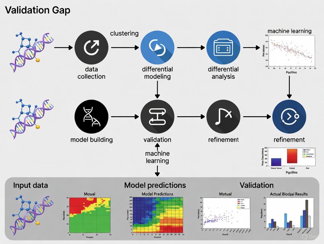
Visualization of the Multi-Modal Data Integration Workflow

Integrating diverse data types is a proven strategy to improve predictive accuracy. The following diagram illustrates a robust workflow for multi-modal data integration and validation in systems biology.

The Scientist's Toolkit: Key Reagents and Computational Solutions

Building and validating a predictive model requires a suite of wet-lab and computational tools. The table below details key resources essential for conducting the experiments and analyses described in this guide.

Table 3: Research Reagent Solutions for Predictive Model Development and Validation

Item / Solution	Function / Application	Example Use-Case
Mass Spectrometry	Enables quantification of thousands of proteins simultaneously, capturing dynamic proteome changes. [1]	Proteome-level validation of predictive models.
Multiplex Immunofluorescence	Provides spatial profiling of the tumor microenvironment, revealing cell organization. [2]	Integrating spatial biology to improve immunotherapy response prediction.
SCORPIO AI Model	Analyzes multi-modal data to predict overall survival; outperforms traditional biomarkers. [2]	A tool for benchmarking new models against state-of-the-art performance.
Python & Scikit-learn	Provides implementations for a wide array of feature selection and classification algorithms. [5]	Building and testing custom predictive models from high-dimensional biological data.
PyBaMM (Python Battery MMM)	An open-source environment for simulating and validating physics-based models against experimental data. [7]	A framework for reproducible model testing and comparison, as demonstrated with battery data.
High-Performance Computing (HPC)	Provides massive computational resources required for big biological data analytics. [8]	Handling tasks like whole-genome sequence alignment and large-scale molecular dynamics.
Cyclopaldic acid	Cyclopaldic acid, CAS:477-99-6, MF:C11H10O6, MW:238.19 g/mol	Chemical Reagent
SCH-202676	SCH-202676, MF:C15H13N3S, MW:267.4 g/mol	Chemical Reagent

Troubleshooting Guide: When Simulation and Data Diverge

A mismatch between simulation and experiment is not a failure but a diagnostic opportunity. Here is a systematic troubleshooting guide based on expert analysis.

• Investigate Data Quality and Model Setup:

  • Re-check Input Parameters: This is the most common source of error. Verify that all biological parameters, boundary conditions, and initial states precisely match the experimental protocol. A subtle error in defining a single parameter can render results completely wrong [3].
  • Re-evaluate Physical/Biological Assumptions: Did the model assume a linear response when the system is non-linear? Was a critical pathway or interaction omitted? Re-evaluating these fundamental choices is key [3] [9].

• Interrogate the Computational Methodology:

  • Assess Mesh/Grid Resolution and Numerical Convergence: In particle-based or spatial models, a coarse mesh is a leading cause of inaccuracy. Perform a Grid Convergence Index (GCI) study to ensure results are independent of numerical discretization [3] [9]. For non-spatial models, ensure the numerical solver has truly converged.
  • Evaluate Feature Selection and Algorithm Choice: The choice of machine learning algorithm and feature selection method significantly impacts performance. Certain pairings are consistently top performers across biological data types [5]. Ensure the chosen turbulence model or classification algorithm is appropriate for the problem's physics/biology [3].

• Address the "Validation Gap" in AI Models:

  • Prioritize External Validation: Always test AI models on independent, external patient cohorts or datasets. This is the only way to identify and address the performance drop that characterizes the validation gap [2].
  • Incorporate Functional Predictions: Move beyond sequence-based screening to function-based algorithms that can flag hazardous or novel functions, thereby closing biosecurity and performance gaps in AI-designed biologics [4].

Visualization of the Model Validation and Troubleshooting Protocol

A systematic protocol is essential for diagnosing and resolving discrepancies between simulation outputs and experimental data. The following flowchart outlines a step-by-step troubleshooting process.

The disconnect between simulation and experimental data remains a fundamental challenge in predictive systems biology. However, as demonstrated through the comparative data and protocols in this guide, this gap can be systematically addressed. The key lies in a rigorous, methodical approach that prioritizes high-quality data, meticulous setup mirroring, and comprehensive quantitative and qualitative validation. The emergence of multi-modal integration and AI, while presenting new challenges like the "validation gap," offers unprecedented opportunities to capture the complexity of biological systems.

For researchers and drug development professionals, closing this gap is critical for translation. It builds the confidence needed to move predictive models from the realm of computational exploration to reliable tools for patient stratification, drug target identification, and guiding personalized therapeutic strategies. By adopting the standards and checklists outlined here, the community can work towards a future where in-silico predictions consistently and accurately inform in-vitro and in-vivo outcomes, accelerating the pace of biomedical discovery.

The promise of predictive systems biology is to use computational models to accurately forecast complex biological behaviors, thereby accelerating therapeutic discovery and biomedical innovation. However, a significant validation gap often separates a model's performance on training data from its real-world predictive power. This gap primarily stems from three interconnected sources: database inconsistencies, missing biological annotations, and model overfitting. These issues compromise the reliability, reproducibility, and generalizability of models, posing a substantial challenge for researchers and drug development professionals. This guide objectively compares the performance of different computational approaches designed to bridge this validation gap, providing a detailed analysis of their underlying methodologies, experimental data, and practical efficacy.

Database Inconsistencies in Ortholog Prediction

Performance Comparison of Ortholog Database Evaluation Methods

Ortholog prediction is fundamental for transferring functional knowledge across species, yet different databases often yield conflicting results. A novel metric, the Signal Jaccard Index (SJI), provides an unsupervised, network-based approach to evaluate these inconsistencies [10]. The table below compares its performance against the common strategy of computing consensus orthologs.

Table 1: Comparison of Methods for Evaluating Ortholog Database Inconsistency

Method Feature	Consensus Orthologs (Common Strategy)	SJI-Based Protein Network [10]
Core Principle	Computes agreement across multiple databases	Applies unsupervised genome context clustering to assess protein similarity
Handling of Inconsistency	Introduces additional arbitrariness	Identifies peripheral proteins in the network as primary sources of inconsistency
Reliability Predictor	Not inherent to the method	Uses degree centrality (DC) in the network to predict protein reliability in consensus sets
Key Advantage	Simple to compute	Objective, avoids arbitrary parameters; DC is stable and unaffected by species selection

Experimental Protocol: SJI Metric and Network Construction

The experimental procedure for implementing the SJI-based evaluation is as follows [10]:

• Calculate Signal Jaccard Index (SJI): Compute the SJI for protein pairs based on unsupervised genome context clustering. This metric serves as a robust measure of protein similarity, rooted in genomic data rather than database annotations.
• Construct Protein Network: Build a comprehensive protein network where nodes represent proteins and edges are weighted based on their calculated SJI similarity values.
• Analyze Network Topology: Analyze the topological features of the constructed network. Proteins located at the network's periphery are identified as the primary contributors to prediction inconsistencies.
• Assess Reliability via Degree Centrality: Calculate the degree centrality for each protein node. This metric serves as a strong, stable predictor of a protein's reliability within consensus ortholog sets.

The following workflow diagram illustrates this experimental protocol:

Missing Annotations in Biochemical Network Models

Performance Comparison of Semantic Propagation Techniques

Missing semantic annotations in network models hinder their comparability, alignment, and reuse. Semantic propagation addresses this by inferring information from annotated, surrounding elements in the network [11]. The table below compares two primary technical approaches.

Table 2: Comparison of Semantic Propagation Methods for Missing Annotations

Method Feature	Feature Propagation (FP)	Similarity Propagation (SP)
Core Principle	Associates each model element with a feature vector describing its relation to biological concepts; vectors are propagated across the network.	Directly propagates pairwise similarity scores between elements from different models based on network structure.
Computational Load	Lower	Higher
Input Requirements	Requires feature vectors derived from annotations.	Can work with any initial similarity measure, not necessarily feature-based.
Output	Inferred feature vectors for all elements, providing an enriched description.	An inferred similarity score for element pairs, used for model alignment.
Typical Application	Predicting missing annotations for a single model.	Aligning two or more models directly.

Experimental Protocol: Model Alignment via SemanticSBML

The protocol for using semantic propagation to align models and predict missing annotations with the semanticSBML tool involves the following steps [11]:

• Model Input: Provide the partially annotated Systems Biology Markup Language (SBML) model(s) as input.
• Choose Propagation Method:
  • For Feature Propagation (FP): Represent each element's annotations as a feature vector. The propagation allows elements to inherit semantic information from their network neighbors.
  • For Similarity Propagation (SP): Define an initial direct similarity (e.g., based on existing annotations). The propagation refines this similarity by considering the similarities of connected elements.
• Execute Propagation: Run the chosen algorithm to compute inferred feature vectors (FP) or inferred similarity scores (SP) for all model elements, including non-annotated ones.
• Perform Model Alignment: Use a greedy heuristic to match elements between models based on the inferred similarities (from SP) or inferred feature vectors (from FP). Elements are grouped into tuples believed to be equivalent.
• Predict Annotations (Optional): For a sparsely annotated model, align it to a fully annotated database (e.g., BioModels). Transfer annotations from the best-matching database element to the non-annotated model element as a suggested prediction.

The logical flow of the similarity propagation method, which is particularly effective for aligning models with poor initial annotations, is shown below:

Model Overfitting in Dynamic Modeling and Immunological Applications

Performance Comparison of Robust Parameter Estimation Strategies

Overfitting occurs when a model learns the noise in the training data rather than the underlying biological signal, leading to poor generalizability. This is a critical concern in dynamic modeling of biological systems and in immunological applications like vaccine response prediction [12] [13]. The table below compares standard and robustified approaches.

Table 3: Comparison of Parameter Estimation Methods to Combat Overfitting

Method Feature	Standard Local Optimization (e.g., MultiStart)	Robust & Regularized Global Optimization [13]
Optimization Scope	Local search, prone to getting trapped in local minima.	Efficient global optimization to handle nonconvexity and find better solutions.
Handling of Ill-Conditioning	Often exacerbates overfitting by finding complex, non-generalizable solutions.	Uses regularization (e.g., Tikhonov, Lasso) to penalize model complexity, reducing overfitting.
Parameter Identifiability	May not adequately address non-identifiable parameters.	Systematically incorporates prior knowledge and handles non-identifiability via regularization.
Bias-Variance Trade-off	Can result in high variance and low bias.	Aims for the best trade-off, producing models with better predictive value.
Key Outcome	Potentially good fit to calibration data, poor generalization.	Improved model generalizability and more reliable predictions on new data.

Experimental Protocol: Regularized Parameter Estimation for Dynamic Models

A robust protocol for parameter estimation in dynamic models, designed to fight overfitting, combines global optimization with regularization [13].

• Problem Formulation: Define the parameter estimation as a nonlinear programming problem (NLP) with differential-algebraic constraints. The cost function (e.g., maximum likelihood) measures the mismatch between model predictions and experimental data.
• Apply Global Optimization: Use an efficient global optimization algorithm to explore the parameter space broadly. This step is crucial to avoid convergence to local minima and to find a region near the global optimum.
• Implement Regularization: Incorporate a regularization term into the cost function. This term penalizes the deviation of parameters from prior knowledge (e.g., from literature or preliminary experiments) or encourages desirable properties like parameter sparsity.
• Cross-Validation: Validate the calibrated model using a new, independent dataset that was not used for parameter estimation. This step is essential for testing the model's predictive power and ensuring that overfitting has been mitigated.

The workflow for this robust calibration strategy is as follows:

Table 4: Key Research Reagents and Computational Tools for Bridging the Validation Gap

Item Name	Function/Application	Specific Utility
semanticSBML [11]	Open-source library and web service for model annotation and alignment.	Performs semantic propagation to predict missing annotations and align partially annotated biochemical network models.
BioModels Database [11]	Curated repository of published, annotated mathematical models of biological processes.	Serves as a reference database for transferring annotations via model alignment and for benchmarking.
Signal Jaccard Index (SJI) [10]	A metric derived from unsupervised genome context clustering.	Evaluates ortholog database inconsistency and constructs a protein network to identify error-prone predictions.
Regularization Algorithms [13]	Computational methods (e.g., Tikhonov, Lasso) that add a penalty to the model's cost function.	Reduces model overfitting by penalizing excessive complexity during parameter estimation, improving generalizability.
Global Optimization Solvers [13]	Numerical software designed to find the global optimum of nonconvex problems (e.g., metaheuristics, scatter search).	Essential for robust parameter estimation in dynamic models, helping to avoid non-physical local solutions.
BioPreDyn-bench Suite [14]	A suite of benchmark problems for dynamic modelling in systems biology.	Provides ready-to-run, standardized case studies for fairly evaluating and comparing parameter estimation methods.

Genome-scale metabolic reconstructions are fundamental for modeling an organism's molecular physiology, correlating its genome with its biochemical capabilities [15]. The reconstruction process translates annotated genomic data into a structured network of biochemical reactions, which can then be converted into mathematical models for simulation, most commonly using Flux Balance Analysis (FBA) [16] [15]. While automated reconstruction tools have been developed to accelerate this process, a significant validation gap persists between the models generated by these automated pipelines and biological reality. This case study examines the specific limitations of automated reconstruction methods, quantifying their performance against manually curated benchmarks and outlining methodologies to bridge this accuracy gap. This validation gap presents a critical challenge for researchers in systems biology and drug development who rely on these models for predictive analysis.

Experimental Protocols for Assessing Reconstruction Accuracy

Evaluating the output of automated reconstruction tools requires rigorous experimental design that compares their predictions against high-quality, manually curated models and experimental data. The following protocols outline standard methodologies used in the field.

Protocol 1: Benchmarking Against Manually Curated Models

This protocol assesses the ability of automated tools to recreate known, high-quality metabolic networks [17] [18].

• Input Preparation: Select a target organism with a high-quality, manually curated genome-scale metabolic model (e.g., Lactobacillus plantarum or Bordetella pertussis) [17].
• Tool Execution: Input the genome sequence of the target organism into multiple automated reconstruction platforms (e.g., CarveMe, ModelSEED, RAVEN, AuReMe) [17].
• Model Comparison: Systematically compare the output draft networks from each tool against the manually curated model. Key comparison metrics include:
  • Reaction Recall: The proportion of reactions in the manual model correctly identified by the automated tool.
  • Reaction Precision: The proportion of reactions in the automated model that are present in the manual model.
  • Gene-Protein-Reaction (GPR) Association Accuracy: The correctness of gene assignments to reactions [17].
• Functional Assessment: Use flux balance analysis to test if the automated model can produce all biomass precursors and achieve growth under defined conditions, similar to the manual model [18].

Protocol 2: Validation Against Experimental Phenotype Data

This protocol tests the predictive power of automated models against empirical data [19].

• Data Curation: Compile large-scale phenotypic data for test organisms. This includes:
  • Carbon Source Utilization: Data on which carbon sources support microbial growth.
  • Enzyme Activity Assays: Results from biochemical tests (e.g., from the Bacterial Diversity Metadatabase - BacDive).
  • Gene Essentiality Data: Information on genes required for growth under specific conditions [19].
• Model Prediction: Use the automated models to simulate the curated phenotypes (e.g., predict growth on different carbon sources or the outcome of gene knockouts).
• Performance Calculation: Calculate standard performance metrics such as False Negative Rate and True Positive Rate by comparing predictions against experimental results [19].

The diagram below illustrates the workflow for a comparative assessment of reconstruction tools, integrating both benchmarking approaches.

Performance Comparison: Automated Tools vs. Manual Curation

Systematic assessments reveal that while automated tools offer speed, they often trail manual curation in accuracy and biological fidelity.

Quantitative Accuracy Metrics

The following table summarizes key performance indicators from published benchmark studies.

Table 1: Quantitative Performance Metrics of Automated Reconstruction Tools

Assessment Metric	Manual Curation (Benchmark)	Automated Tools (Range)	Key Findings
Gap-Filling Accuracy (Precision)	Not Applicable (Reference)	66.6% (GenDev on B. longum) [18]	Automated gap-filling introduced false-positive reactions; manual review is essential.
Gap-Filling Accuracy (Recall)	Not Applicable (Reference)	61.5% (GenDev on B. longum) [18]	Automated methods missed ~40% of reactions identified by human experts.
Enzyme Activity Prediction (True Positive Rate)	Not Applicable (Reference)	27% - 53% (CarveMe: 27%, ModelSEED: 30%, gapseq: 53%) [19]	Performance varies significantly between tools; gapseq showed notably higher accuracy.
Reaction Network Completeness	Varies by model (Reference)	Variable and tool-dependent [17]	No single tool outperforms all others in every defined feature.

Limitations in Pathway and Context Prediction

Beyond quantitative metrics, automated tools struggle with specific qualitative aspects:

• Incorrect Inference of Metabolic Pathways: Automated reconstructions can generate manifold paths that require expert manual verification to accept some and reject most others [20]. This is often due to over-reliance on genomic annotations without sufficient biochemical context.
• Lack of Organism-Specific Context: Parsimony-based gap-fillers may select reactions from a database at random when multiple, equally "costed" options exist, potentially missing the biologically relevant one. A case study on B. longum showed an automated tool selecting one of four possible reactions for L-asparagine synthesis, while manual curation correctly identified the specific reaction based on the presence of other pathway enzymes [18].
• Dependence on Input Database Quality: The accuracy of any tool is constrained by the completeness and quality of the reaction database it uses. Inconsistent atom mapping or energy-generating futile cycles in databases can lead to functionally incorrect models [19] [18].

The diagram below outlines the specific stages where errors are introduced during automated reconstruction and how they are typically addressed in manual curation.

The Scientist's Toolkit: Key Research Reagents & Databases

Successful metabolic reconstruction, whether automated or manual, relies on a core set of databases and software tools. The table below catalogs essential resources for the field.

Table 2: Essential Research Reagents and Databases for Metabolic Reconstruction

Resource Name	Type	Primary Function in Reconstruction	Relevance to Validation
KEGG [15]	Database	Provides reference information on genes, proteins, reactions, and pathways.	Serves as a primary data source for many automated tools; a standard for pathway analysis.
MetaCyc [17] [15]	Database	A curated encyclopedia of experimentally defined metabolic pathways and enzymes.	Used as a high-quality reference database for reconstruction and manual curation.
BiGG Models [17] [15]	Database	A knowledgebase of genome-scale metabolic reconstructions.	Provides access to existing curated models for use as templates or benchmarks.
BRENDA [15]	Database	A comprehensive enzyme information system.	Used to verify enzyme function and organism-specific enzyme activity.
Pathway Tools [17] [15]	Software Suite	Assists in building, visualizing, and analyzing pathway/genome databases.	Used for both automated and semi-automated reconstruction and curation.
CarveMe [17] [19]	Software Tool	Automated reconstruction using a top-down approach from a universal model.	Known for generating "ready-to-use" models for FBA; often used in performance comparisons.
ModelSEED [17] [19]	Software Tool	Web-based resource for automated reconstruction and analysis of metabolic models.	Often benchmarked for phenotype prediction accuracy.
gapseq [19]	Software Tool	Automated tool for predicting metabolic pathways and reconstructing models.	Recently developed tool shown to improve prediction accuracy for bacterial phenotypes.
Resorcinomycin A	Resorcinomycin A, CAS:100234-70-6, MF:C14H20N4O5, MW:324.33 g/mol	Chemical Reagent	Bench Chemicals
Griseolutein B	Griseolutein B, CAS:2072-68-6, MF:C17H16N2O6, MW:344.32 g/mol	Chemical Reagent	Bench Chemicals

This case study demonstrates that a significant validation gap exists between automated and manually curated metabolic reconstructions. Quantitative benchmarks reveal that even state-of-the-art automated tools can exhibit low precision and recall in gap-filling and show variable performance in predicting enzymatic capabilities [18] [19]. The core limitations stem from a lack of biological context, inherent database inaccuracies, and the inability of algorithms to incorporate the expert knowledge that guides manual curation [20] [21] [18].

To bridge this gap, the future of metabolic reconstruction lies in hybrid approaches that integrate the scalability of automation with the precision of manual curation. Promising strategies include leveraging manually curated models as templates for related organisms [21], developing improved algorithms that incorporate more biological evidence (e.g., as seen in gapseq [19]), and establishing more robust standardized protocols for model validation. For researchers in drug development and systems biology, these findings underscore the critical importance of critically evaluating and manually refining automatically generated models before using them for critical predictions.

Unanticipated off-target effects represent a critical challenge in drug discovery, directly contributing to high rates of clinical attrition and the failure of promising therapeutic candidates. These effects, defined as a drug's action on gene products other than its intended target, are a principal cause of adverse reactions and toxicity that derail development programs, particularly in Phase II and III trials [22] [23]. The validation gap in predictive systems biology—where computational models fail to generalize outside their development cohort—severely limits our ability to foresee these effects, resulting in costly late-stage failures [2]. This guide compares the primary methodological approaches for predicting off-target effects, evaluates their performance in anticipating clinical attrition, and details the experimental protocols that underpin this critical field. As drug discovery expands into novel modalities like PROTACs, oligonucleotides, and cell/gene therapies, each with unique off-target profiles, robust and predictive preclinical profiling becomes indispensable for improving the dismal likelihood of approval (LOA), which stands at just 5-7% for small molecules [24] [25].

Quantifying the Clinical Attrition Problem

High attrition rates, especially in Phase II, plague drug development across all modalities. The table below summarizes global clinical attrition data, illustrating the stark reality of drug development failure.

Table 1: Global Clinical Attrition Rates by Drug Modality (2005-2025)

Modality	Phase I → II Success	Phase II → III Success	Phase III → Approval Success	Overall LOA
Small Molecules	52.6%	28.0%	~57.0%	~6.0%
Monoclonal Antibodies (mAbs)	54.7%	Information Missing	68.1%	12.1%
Antibody-Drug Conjugates (ADCs)	41.0%	42.0%	Information Missing	Information Missing
Protein Biologics (non-mAbs)	51.6%	Information Missing	89.7%	9.4%
Peptides	52.3%	Information Missing	Information Missing	8.0%
Oligonucleotides (ASOs)	61.0%	Information Missing	Information Missing	5.2%
Oligonucleotides (RNAi)	~70.0%	Information Missing	~100%	13.5%
Cell & Gene Therapies (CGTs)	48-52%	Information Missing	Information Missing	10-17%

Data compiled from industry analyses (Biomedtracker/PharmaPremia) show that despite differences in modality, Phase II is the most significant hurdle, with the majority of programs failing at this stage due to efficacy and safety concerns, the latter often linked to unanticipated off-target effects [25].

Comparative Analysis of Predictive Methodologies for Off-Target Effects

A range of computational and experimental methods has been developed to predict off-target effects early in the drug discovery process. Their performance and applicability vary significantly.

Table 2: Performance Comparison of Off-Target Prediction and Profiling Methods

Methodology	Key Principle	Reported Performance	Primary Application	Key Limitations
In silico Bayesian Models [22]	Builds probabilistic models from chemical structure and known pharmacology data to predict binding.	93% ligand detection (IC₅₀ ≤10µM); 94% correct classification rate.	Early-stage compound screening and triage.	Highly dependent on the quality and breadth of training data.
Direct Side-Effect Modeling [22]	Predicts adverse drug reactions directly from chemical structure, bypassing mechanistic knowledge.	90% of known ADRs detected; 92% correct classification.	Late-stage lead optimization and safety profiling.	Model interpretability and back-projection to structure can be challenging.
Comprehensive Experimental Mapping (EvE Bio) [23]	Empirically tests ~1,600 FDA-approved drugs against a vast panel of human cellular receptors.	Provides direct, empirical interaction data, not a prediction. Creates a foundational dataset.	Drug repurposing, polypharmacology, and model validation.	Resource-intensive; limited to existing approved drugs and selected receptors.
AI/Machine Learning Models [2]	Integrates high-dimensional clinical, molecular, and imaging data to uncover complex patterns.	AUC of 0.76 for overall survival (SCORPIO model); 81% predictive accuracy (LORIS model).	Personalized therapy prediction, particularly in oncology.	Prone to a "validation gap," with performance dropping on external datasets.

The convergence of computational and empirical methods is key to closing the validation gap. For instance, the large-scale experimental data generated by efforts like EvE Bio provides the ground-truth data needed to train and validate more robust AI and Bayesian models [22] [23].

Detailed Experimental Protocols for Off-Target Profiling

Protocol 1: In silico Bayesian Model Building for Target Prediction

This protocol outlines the creation of computational models to predict a compound's binding to preclinical safety pharmacology (PSP) targets [22].

• Data Curation: Compile a comprehensive dataset of chemical structures and their associated in vitro binding affinities (e.g., ICâ‚…â‚€ values) for a panel of 70+ PSP-related targets.
• Descriptor Calculation: For each compound, calculate numerical descriptors that encode its chemical structure and properties.
• Model Training: For each PSP target, train a separate Bayesian machine learning model. The model learns the probabilistic relationship between the chemical descriptors and the likelihood of binding.
• Model Validation: Validate model performance using held-out test data not seen during training. Key metrics include sensitivity (ability to detect true binders) and overall correct classification rate.
• Deployment & Interpretation: Use the trained models to screen virtual or real compound libraries. The features of the model are interpretable and can be back-projected to chemical structure, suggesting which structural motifs contribute to off-target binding [22].

Protocol 2: Large-Scale Empirical Off-Target Mapping

This protocol describes the systematic, experimental approach to mapping drug-target interactions, as employed by organizations like EvE Bio [23].

• Receptor Panel Selection: Curate a diverse panel of hundreds of clinically important human cellular receptors representing a wide range of target classes (e.g., GPCRs, kinases, ion channels).
• Compound Library Curation: Assemble a library of approximately 1,600 FDA-approved drugs.
• High-Throughput Binding Assays: Subject each drug in the library to a standardized, high-throughput binding assay against every receptor in the panel. This measures the strength of interaction (e.g., binding affinity) between the drug and receptor.
• Data Collection and Quality Control: Systematically collect the interaction data, implementing rigorous quality controls to ensure reproducibility.
• Data Integration and Curation: Compile the results into a centralized, searchable database that maps every drug to all its detected receptor interactions, both intended (on-target) and unintended (off-target).
• Data Release: The final dataset is released under a non-commercial, creative commons license (CC-NA) for academic use, and is available for commercial licensing [23].

The following diagram illustrates the workflow for this large-scale empirical mapping process.

Diagram 1: Empirical off-target mapping workflow.

The Scientist's Toolkit: Key Research Reagent Solutions

The following table details essential reagents and resources used in the experimental profiling of off-target effects.

Table 3: Key Research Reagents for Off-Target Effect Profiling

Reagent / Resource	Function in Experimental Protocol
Preclinical Safety Pharmacology (PSP) Target Panel [22]	A curated set of 70+ in vitro binding assays (e.g., for GPCRs, kinases) used to screen compounds for potential adverse effects.
FDA-Approved Drug Library [23]	A comprehensive collection of ~1,600 approved small molecule drugs, used for large-scale repurposing and off-target screening.
Human Cellular Receptor Library [23]	A diverse panel of hundreds of cloned human receptors, enabling systematic profiling of compound interactions.
Positional Weight Matrix (PWM) [26]	A de facto standard model for transcription factor (TF) DNA binding specificity, used in benchmarking studies.
Mass Spectrometry Platforms	Enables the quantification of thousands of proteins simultaneously for proteome-wide validation of model predictions [1].
Gostatin	Gostatin, CAS:78416-84-9, MF:C8H10N2O5, MW:214.18 g/mol
Andrimid	Andrimid

Analysis of the Validation Gap in Predictive Systems Biology

A persistent "validation gap" undermines the reliability of predictive models in biology. This gap is the failure of models, including those for off-target effects and therapy response, to maintain their performance when applied to independent, external datasets [2]. For example, while AI models for immunotherapy response can achieve AUCs >0.9 in controlled research settings, their performance often drops significantly in real-world clinical cohorts [2].

The causes of this gap are multifaceted and create a logical flow of challenges, from data input to real-world application, as shown below.

Diagram 2: The validation gap challenge in predictive modeling.

Closing this validation gap requires a multi-faceted approach, including the generation of large-scale, high-quality empirical datasets (like those from EvE Bio) for model training and benchmarking [26] [23], the adoption of international data standardization frameworks [2], and rigorous external validation practices before clinical implementation [26] [2].

The integration of multi-omics data represents a transformative frontier in systems biology, promising a comprehensive understanding of how molecular interactions across biological scales govern phenotype manifestation. Despite unprecedented growth in the field—with multi-omics scientific publications more than doubling in just two years (2022–2023)—a significant validation gap persists between computational predictions and physiological reality [27]. Current machine learning methods primarily establish statistical correlations between genotypes and phenotypes but struggle to identify physiologically significant causal factors, limiting their predictive power for unprecedented perturbations [28] [29]. This gap stems from several interconnected challenges: scarcity of labeled data for supervised learning, generalization across biological domains and species, disentangling causation from correlation, and the inherent difficulties in integrating heterogeneous data types with varying dimensions, measurement units, and noise structures [28] [30].

The validation challenge is particularly acute in translational applications such as drug development, where over 90% of approved medications originated from phenotype-based discovery, yet target-based approaches dominated by artificial intelligence (AI) often fail to produce clinically effective treatments [28] [31]. Bridging this gap requires not only advanced computational methods but also robust experimental designs, standardized reference materials, and biological interpretability built into model architectures. This review examines emerging approaches that address these challenges through innovative integration strategies, with particular focus on their validation frameworks and comparative performance in predictive systems biology.

Comparative Analysis of Multi-Omics Integration Approaches

AI-Driven Multi-Scale Predictive Modeling

Overview and Methodology: AI-powered biology-inspired multi-scale modeling represents a paradigm shift from correlation-based to causation-aware predictive modeling. This framework integrates multi-omics data across three critical dimensions: (1) biological levels (genomics, transcriptomics, proteomics, metabolomics), (2) organism hierarchies (cell, tissue, organ, organism), and (3) species (model organisms to humans) [28] [29] [32]. The methodology employs endophenotypes—molecular intermediates such as RNA expression, protein modifications, and metabolite concentrations—as mechanistic bridges connecting genetic determinants to organismal phenotypes [28]. Unlike conventional machine learning that treats biological systems as black boxes, this approach structures AI architectures around known biological hierarchies and prior knowledge, enabling more physiologically realistic predictions.

Experimental Validation and Performance: Validation of this approach utilizes perturbation functional omics profiling from resources like TCGA, LINCS, DepMap, and scPerturb which provide labeled data for supervised learning [28]. These datasets systematically capture molecular responses to genetic and chemical perturbations, creating ground truth benchmarks for model assessment. For example, scPerturb integrates 44 public single-cell perturbation datasets with CRISPR and drug interventions, providing single-cell resolution for quantifying heterogeneous cellular responses [28]. The Table 1 summarizes the experimental data resources available for developing and validating multi-omics integration models.

Table 1: Key Data Resources for Multi-Omics Model Validation

Resource	Perturbation Types	Molecular Profiling	Key Applications
TCGA [28] [33]	Drug treatments	Genomic, transcriptomic, epigenomic, proteomic	Cancer biomarker identification, therapeutic target discovery
LINCS [28]	Drug, CRISPR-Cas9, ShRNA	Transcriptomic, proteomic, kinase binding, cell viability	Cellular signature analysis, drug mechanism of action
DepMap [28] [33]	CRISPR-Cas9, RNAi, drug	Genomic, transcriptomic, proteomic, drug sensitivity	Cancer dependency mapping, drug response prediction
scPerturb [28]	CRISPR, cytokines, drugs	Single-cell RNA-seq, proteomic, epigenomic	Single-cell perturbation response, cellular heterogeneity
PharmacoDB [28]	Drug	Genomic, transcriptomic, proteomic	Drug sensitivity analysis, personalized medicine
Quartet Project [34]	Built-in family pedigree	DNA, RNA, protein, metabolites	Multi-omics reference materials, data integration QC

Advantages and Limitations: The key advantage of AI-driven multi-scale modeling is its ability to generalize predictions across biological contexts and identify causal mechanisms rather than mere correlations [28] [31]. The framework shows particular promise for phenotype-based drug discovery, where perturbation functional omics provides quantitative, mechanistic readouts for compound screening [28]. However, limitations include high computational complexity, dependence on extensive and diverse training data, and challenges in interpreting complex network architectures. Validation remains particularly difficult for human-specific predictions where in vivo data is scarce or ethically constrained.

Reference Material-Based Frameworks for Validation

Overview and Methodology: The Quartet Project addresses a fundamental challenge in multi-omics integration: the lack of ground truth for method validation [34]. This approach provides publicly available suites of multi-omics reference materials derived from immortalized cell lines from a family quartet (parents and monozygotic twin daughters). The methodology employs a ratio-based profiling approach that scales absolute feature values of study samples relative to a concurrently measured common reference sample, enabling reproducible and comparable data across batches, laboratories, and platforms [34]. The family structure provides built-in truth defined by genetic relationships and central dogma information flow from DNA to RNA to protein.

Experimental Validation and Performance: The Quartet reference materials have been comprehensively characterized across multiple platforms: 7 DNA sequencing platforms, 2 RNA-seq platforms, 9 proteomics platforms, and 5 metabolomics platforms [34]. Performance is quantified using two specialized metrics: (1) sample classification accuracy (ability to distinguish the four individuals and three genetic clusters), and (2) central dogma conformity (correct identification of cross-omics feature relationships following DNA→RNA→protein information flow). The ratio-based method demonstrates superior reproducibility compared to absolute quantification, which is identified as the root cause of irreproducibility in multi-omics measurement [34].

Table 2: Quartet Project Reference Materials and Applications

Reference Material	Source	Key Characteristics	Primary Applications
DNA Reference	B-lymphoblastoid cell lines	Mendelian inheritance patterns, variant calling validation	Genomic technology proficiency testing
RNA Reference	Matched to DNA samples	Expression quantification, splice variant analysis	Transcriptomic platform benchmarking
Protein Reference	Same cell lines as nucleic acids	Post-translational modifications, abundance measurements	Proteomic method validation
Metabolite Reference	Same cell lines as other omics	Small molecule profiles, pathway analysis	Metabolomic standardization

Advantages and Limitations: The Quartet framework provides an essential validation tool for closing the verification gap in multi-omics integration, offering objective quality control metrics and reference standards for technology benchmarking [34]. Its ratio-based approach facilitates integration across diverse datasets and platforms. Limitations include potential context-specific performance (e.g., cancer vs. non-cancer applications) and the challenge of extending insights to more complex tissues and clinical samples. Nevertheless, it represents a crucial step toward standardized validation in multi-omics research.

Biologically Interpretable Neural Networks

Overview and Methodology: Visible neural networks represent an emerging approach that embeds prior biological knowledge into network architectures to enhance both prediction accuracy and interpretability [35]. These networks structure layers according to biological hierarchies—connecting input features to genes, genes to pathways, and pathways to phenotypes—making the decision-making process transparent and biologically meaningful [35]. In one implementation, multi-omics data (transcriptomics and methylomics) are integrated at the gene level, with CpG methylation sites annotated to genes based on genomic distance and combined with expression data in the gene layer [35].

Experimental Validation and Performance: This approach has been validated using the BIOS consortium dataset (N=2940) for predicting smoking status, age, and LDL levels [35]. In cohort-wise cross-validation, the method demonstrated consistently high performance for smoking status prediction (mean AUC: 0.95), with interpretation revealing biologically relevant genes such as AHRR, GPR15, and LRRN3 [35]. Age was predicted with a mean error of 5.16 years, with genes COL11A2, AFAP1, and OTUD7A consistently predictive. For both regression tasks, multi-omics networks improved performance, stability, and generalizability compared to single-omic networks [35]. The Table 3 summarizes the performance metrics across different prediction tasks.

Table 3: Performance of Biologically Interpretable Neural Networks on Multi-Omics Data

Prediction Task	Performance Metric	Key Predictive Features	Generalizability Across Cohorts
Smoking Status	AUC: 0.95 (95% CI: 0.90-1.00)	AHRR, GPR15, LRRN3 methylation	High consistency across 4 cohorts
Subject Age	Mean error: 5.16 years (95% CI: 3.97-6.35)	COL11A2, AFAP1, OTUD7A expression	Moderate variability between cohorts
LDL Levels	R²: 0.07 (single cohort)	Complex multi-omic interactions	Limited generalizability across cohorts

Advantages and Limitations: The primary advantage of visible neural networks is their ability to combine predictive power with biological interpretability, generating testable hypotheses about mechanistic relationships [35]. The structured architecture also regularizes the model, reducing overfitting and improving generalization across cohorts. Limitations include dependence on accurate prior knowledge annotations, potentially missing novel biological relationships not captured in existing databases, and sensitivity to weight initializations that can affect interpretation stability [35].

Experimental Protocols for Multi-Omics Integration

Standardized Workflow for Multi-Omics Study Design

Recent research has identified nine critical factors that fundamentally influence multi-omics integration outcomes, providing an evidence-based framework for experimental design [30]. These factors are categorized into computational aspects (sample size, feature selection, preprocessing strategy, noise characterization, class balance, number of classes) and biological aspects (cancer subtype combinations, omics combinations, clinical feature correlation). Benchmark tests across ten cancer types from TCGA revealed that robust performance requires: ≥26 samples per class, selection of <10% of omics features, sample balance under 3:1 ratio, and noise levels below 30% [30]. Feature selection alone improved clustering performance by 34%, highlighting its critical importance in study design.

Protocol for Cross-Species Multi-Omics Integration

Integrating multi-omics data across species requires specialized methodologies to address evolutionary divergence while leveraging conserved biological mechanisms [28] [31]. The protocol involves: (1) Orthology mapping using standardized gene annotation databases, (2) Conserved pathway identification focusing on evolutionarily stable biological processes, (3) Cross-species normalization to account for technical and biological variations, and (4) Transfer learning where models pre-trained on model organisms are fine-tuned with human data [28]. This approach is particularly valuable for drug discovery, where model organisms provide perturbation response data that can be translated to human contexts through multi-omics alignment [31].

Visualization of Multi-Omics Integration Approaches

Workflow for Reference Material-Based Multi-Omics Integration

Quartet Project Multi-Omics Integration Workflow

Architecture of Biologically Interpretable Neural Networks

Visible Neural Network Architecture

Table 4: Key Research Reagent Solutions for Multi-Omics Integration

Resource Type	Specific Examples	Function and Application	Key Characteristics
Reference Materials	Quartet Project references [34]	Method validation, cross-platform standardization	Built-in ground truth from family pedigree
Data Repositories	TCGA, ICGC, CCLE, CPTAC [28] [33]	Model training, benchmarking, validation	Clinical annotations, multiple cancer types
Perturbation Databases	LINCS, DepMap, scPerturb [28]	Causal inference, mechanism of action studies	Genetic and chemical perturbations
Bioinformatics Tools	GenNet, P-net, MOFA [35]	Data integration, visualization, interpretation	Biologically informed architectures
Quality Control Metrics	Mendelian concordance, SNR, classification accuracy [34]	Performance assessment, method selection	Objective benchmarking criteria

The integration of multi-omics data for holistic model building represents one of the most promising avenues for advancing predictive systems biology, yet significant challenges remain in validation and translational application. The emerging approaches discussed—AI-driven multi-scale modeling, reference material frameworks, and biologically interpretable neural networks—each contribute distinct strategies for addressing the validation gap. The AI-driven framework excels in cross-domain generalization and causal inference, reference materials provide essential ground truth for method benchmarking, and visible neural networks offer unprecedented interpretability while maintaining predictive power.

The future of multi-omics integration lies in combining the strengths of these approaches—developing biologically informed AI models validated against standardized reference materials and interpreted through transparent architectures. As these methodologies mature and converge, they hold immense potential for illuminating fundamental principles of biology and accelerating the discovery of novel therapeutic targets, biomarkers, and personalized treatment strategies for presently intractable diseases. Critical to this progress will be continued development of robust validation frameworks that bridge the gap between computational predictions and physiological reality, ultimately fulfilling the promise of multi-omics integration in predictive systems biology.

Advanced Methodologies for Building Biologically Relevant Predictive Models

Predictive modeling in systems biology seeks to translate mathematical abstractions of biological systems into reliable tools for understanding cellular behavior, disease mechanisms, and therapeutic development [36] [1]. A persistent challenge, however, is the validation gap – the discrepancy between a model's theoretical predictions and its real-world biological accuracy. This gap often originates during the creation of genome-scale metabolic models, which are typically derived from annotated genomes and are invariably incomplete, lacking fully connected metabolic networks due to undetected enzymatic functions [18]. Gap filling, the computational process of proposing additional reactions to enable production of all essential biomass metabolites, is therefore a critical step in making these models biologically plausible and functionally useful.

Traditionally, automated gap filling has relied on parsimony-based principles, which seek minimal sets of reactions to connect metabolic networks. However, these methods can propose biochemically inaccurate solutions and struggle with numerical instability [18]. Emerging likelihood-based approaches offer a more statistically rigorous framework by directly quantifying parameter and prediction uncertainty, propagating measurement errors through model predictions, and providing confidence intervals for model outputs [37] [38]. This guide compares these methodological paradigms, providing experimental data and protocols to help researchers select appropriate strategies for bridging the validation gap in their predictive systems biology research.

Methodological Comparison: Parsimony vs. Likelihood-Based Approaches

Core Principles and Implementation

Parsony-based gap filling operates on the principle of metabolic frugality, seeking the smallest number of non-native reactions required to enable network functionality, typically using Mixed-Integer Linear Programming (MILP) solvers. In practice, tools like the GenDev algorithm within Pathway Tools identify minimum-cost solutions to complete metabolic networks, often using reaction databases like MetaCyc as candidate pools [18].

In contrast, likelihood-based approaches utilize the prediction profile likelihood to quantify how well different model predictions or parameter values agree with experimental data. This method performs constraint optimization of the likelihood function for fixed prediction values, effectively testing the agreement of predicted values with existing measurements. The resulting confidence intervals accurately reflect parameter uncertainty and can identify non-observable model components [37]. This framework is particularly valuable for dynamic models of biochemical networks where parameters are estimated from experimental data and nonlinearity hampers uncertainty propagation [37].

Experimental Performance Comparison

A direct comparison of parsimony-based automated gap filling versus manually curated solutions reveals significant accuracy differences. In a study constructing a metabolic model for Bifidobacterium longum subsp. longum JCM 1217, researchers evaluated the performance of the GenDev gap filler against expert manual curation [18].

Table 1: Performance Metrics of Gap-Filling Approaches

Metric	Parsimony-Based (GenDev)	Manually Curated Solution
Reactions Added	12 (10 minimal after analysis)	13
True Positives	8	13
False Positives	4	0
False Negatives	5	0
Recall	61.5%	100%
Precision	66.6%	100%

The analysis revealed several critical limitations of the parsimony approach. The GenDev solution was not minimal – two reactions could be removed while maintaining functionality, indicating numerical precision issues with the MILP solver. Furthermore, several proposed reactions were biochemically implausible for the organism's anaerobic lifestyle, highlighting how purely mathematical solutions may lack biological fidelity [18].

Likelihood-based methods address these limitations by incorporating statistical measures of confidence and compatibility with experimental data. In parameter estimation for dynamic models, maximum likelihood approaches have demonstrated 4x greater accuracy and required 200x less computational time compared to simulation-based methods [39]. This efficiency gain is particularly valuable for large-scale models common in systems biology research.

Table 2: Technical Characteristics of Gap-Filling Approaches

Characteristic	Parsimony-Based Approach	Likelihood-Based Approach
Objective Function	Minimal reaction count	Maximum likelihood agreement with data
Uncertainty Quantification	Limited	Comprehensive (profile likelihood)
Biological Context	Often ignored	Incorporates taxonomic range, directionality
Numerical Stability	MILP solver precision issues	Robust optimization frameworks
Handling Non-identifiable Parameters	Poor	Excellent (interpreted as non-observability)
Implementation Complexity	Moderate	High (requires statistical expertise)

Experimental Protocols for Method Evaluation

Protocol for Parsimony-Based Gap Filling

The following protocol was used in the B. longum gap-filling evaluation [18]:

• Input Preparation: Start with a gapped Pathway/Genome Database (PGDB) containing the predicted reactome and metabolic pathways derived from genome annotation.
• Growth Requirements Definition: Specify the complete set of biomass metabolites (53 in the B. longum study) and nutrient compounds available to the model.
• Gap Analysis: Use flux balance analysis (FBA) to identify which biomass metabolites cannot be produced from the available nutrients.
• Reaction Candidate Pool: Access a biochemical reaction database (e.g., MetaCyc) containing known metabolic reactions with taxonomic range and directionality information.
• Optimization Execution: Run the GenDev algorithm or similar parsimony-based gap filler to identify the minimum-cost set of reactions to enable production of all biomass metabolites.
• Solution Validation: Iteratively test the necessity of each added reaction by removing it and rechecking growth capability using FBA.

Protocol for Likelihood-Based Assessment

For likelihood-based uncertainty quantification in dynamic models, the following methodology is recommended [37]:

• Model Specification: Define the dynamic model structure, typically as a system of ordinary differential equations: ẋ(t) = f(x, p, u), where p represents model parameters and u represents experimental perturbations.
• Observable Definition: Specify the mapping from model states to measurable quantities: y(t) = g(x(t), s_obs) + ε, where ε represents measurement error.
• Likelihood Function Calculation: Compute the log-likelihood for the model parameters given experimental data, typically assuming Gaussian errors: -2LL(y\|θ) = Σi [yi - F(t_i, u, θ)]²/σ² + constant.
• Prediction Profile Likelihood: For a specific prediction z = F(Dpred, θ), optimize the likelihood over parameters satisfying the constraint F(Dpred, θ) = z: PPL(z) = max{θ∈{θ\|F(Dpred, θ)=z}} LL(y\|θ).
• Confidence Interval Calculation: Determine prediction confidence intervals by thresholding the prediction profile likelihood: PCIα(Dpred\|y) = {z \| -2PPL(z) ≤ -2LL*(y) + icdf(χ₁², α)}.

Visualization of Method Workflows

Likelihood-Based Gap Filling and Validation Framework

This workflow illustrates how likelihood-based approaches integrate statistical rigor throughout the gap-filling process, from initial model assessment to experimental validation.

Table 3: Key Computational Tools for Advanced Gap Filling

Tool/Platform	Function	Application Context
Pathway Tools with MetaFlux	Metabolic modeling and parsimony-based gap filling	Genome-scale metabolic reconstruction [18]
Data2Dynamics (Matlab)	Parameter estimation and uncertainty analysis	Likelihood-based assessment and prediction profiles [37] [38]
R/Bioconductor	Statistical computing and multi-omics analysis	General statistical analysis for systems biology [40]
CellDesigner	Graphical modeling of biological networks	Model creation and visualization [40]
BioModels Database	Repository of mathematical models	Model sharing and validation [40]
PyTorch/TensorFlow	Automatic differentiation frameworks	Efficient maximum likelihood estimation [39]
STRINGS, KEGG, Reactome	Pathway databases and interaction networks	Biological context for candidate reactions [40] [41]

The transition from parsimony-based to likelihood-based gap filling represents a significant methodological evolution in predictive systems biology. While parsimony approaches provide computationally efficient solutions, their limited statistical foundation and susceptibility to biochemical inaccuracy (evidenced by 61.5% recall and 66.6% precision rates) present substantial limitations for rigorous model validation [18].

Likelihood-based approaches, through the prediction profile likelihood framework, offer comprehensive uncertainty quantification, robust handling of non-identifiable parameters, and statistically accurate confidence intervals for model predictions [37]. The implementation of these methods in open-source toolboxes like Data2Dynamics makes them increasingly accessible to the research community [38].

For researchers and drug development professionals addressing the validation gap in predictive modeling, we recommend a hybrid approach: using parsimony-based methods for initial network completion followed by likelihood-based assessment for rigorous statistical validation. This combined strategy leverages the computational efficiency of parsimony methods while incorporating the statistical rigor needed for robust, biologically faithful models capable of generating reliable predictions for therapeutic development and basic biological discovery.

The accurate assessment of an individual's biological age (BA) is a cornerstone of predictive systems biology, offering profound insights into healthspan, disease risk, and mortality. However, a significant validation gap persists between model development and their proven utility in predicting clinically relevant outcomes. Many existing BA estimation models are anchored to chronological age (CA) and trained on homogeneous cohorts, limiting their generalizability and clinical applicability for risk stratification [42]. The emergence of transformer-based architectures represents a paradigm shift, directly addressing this gap by integrating multifaceted health data, including morbidity and mortality, to produce BA estimates with superior prognostic power and clinical relevance.

Performance Benchmarking: Transformer Models vs. Established Alternatives

Extensive benchmarking studies demonstrate that transformer-based models consistently outperform conventional biological age estimation methods, particularly in predicting adverse health outcomes.

Table 1: Comparative Performance of Biological Age Estimation Models in Predicting Mortality

Model Type	Data Modality	Key Performance Metric	Result	Context / Cohort
Transformer BA-CA Gap Model [42]	Routine clinical checkups (41-88 features)	Mortality Risk Stratification	Stronger discrimination in men; clear trend in women	151,281 adults, 2003-2020
Gradient Boosting Model [43] [44]	27 clinical factors from checkups	Mean Squared Error (MSE)	4.219	28,417 super-controls
LLM-based BA Model [45]	Health examination reports	Concordance Index (C-index) for All-Cause Mortality	0.757 (95% CI 0.752-0.761)	>10 million participants across 6 cohorts
CT-Based Biological Age (CTBA) Model [46]	Automated CT biomarkers	10-Year AUC for Longevity	0.880	123,281 adults (mean age 53.6)
Demographics Model (Age, Sex, Race) [46]	Chronological Age, Sex, Race	10-Year AUC for Longevity	0.779	Same cohort as CTBA model
Klemera and Doubal's Method [42]	Limited clinical parameters	Mortality Risk Stratification	Underperformed transformer model	Comparative study on 151,281 adults

Table 2: Model Performance in Discriminating Health Status

Model Type	Ability to Distinguish Normal, Pre-disease, Disease	Key Strengths	Interpretability Features
Transformer BA-CA Gap Model [42] [47]	Excellent, with a clear BA gap gradient	Integrates morbidity/mortality; superior risk stratification	Model attention mechanisms
Gradient Boosting Model [43] [44]	Not explicitly tested for this spectrum	High predictive accuracy (R²=0.967) in healthy cohorts	SHAP analysis identifies key markers (kidney function, HbA1c)
LLM-based BA Model [45]	Strongly associated with aging-related phenotypes	Predicts 270 disease risks; organ-specific aging assessment	Interpretability analyses of decision-making process
CT-Based Biological Age (CTBA) Model [46]	N/A (focused on longevity)	Phenotypic; opportunistically derived from existing CTs	Explainable AI algorithms; biomarker contribution quantified

Experimental Protocols and Methodologies

A critical step in validating any predictive model is a rigorous and transparent experimental protocol. The following methodologies from key studies highlight the structured approach required to minimize the validation gap.

• Cohort Design: A retrospective analysis of 151,281 adults aged ≥18 from the Seoul National University Hospital Healthcare System Gangnam Center (2003-2020). Participants were classified into normal, predisease, and disease groups based on comorbidities (diabetes mellitus, hypertension, dyslipidemia) to test the model across a clinical spectrum.
• Data Preprocessing: Features with ≥50% missing data were excluded. Remaining missing values were imputed using the mean. This pragmatic approach managed a large, complex dataset but may reduce variability.
• Model Architecture & Training: A custom transformer model was designed to simultaneously learn multiple objectives:
  • Input Feature Reconstruction
  • BA and CA Alignment
  • Health Status Discrimination
  • Mortality Prediction
  • Training leveraged unsupervised and self-supervised strategies, avoiding over-reliance on CA as a primary anchor.
• Validation & Comparison: Model performance was compared against established methods (Klemera and Doubal’s method, CA cluster-based model, deep neural network) by analyzing BA gap distributions, health status stratification, and mortality prediction via Kaplan-Meier analyses.

• Cohort and "Ground Truth" Definition: Models were trained on a "super-control" cohort (n=28,417) from the H-PEACE study, selected for the absence of diseases like diabetes and hypertension, and excluding smokers and drinkers. This defines the assumption that chronological age aligns with biological age in physiologically standard individuals.
• Feature Set: 27 routinely available clinical factors, including demographics, anthropometrics, metabolic panels, liver function tests, and complete blood count.
• Model Training & Evaluation: Eight machine learning models were evaluated using 5-fold cross-validation. Performance was assessed via Adjusted R² and Mean Squared Error (MSE).
• Interpretability: SHapley Additive exPlanations (SHAP) analysis was conducted to identify significant predictors of biological age, such as kidney function markers, gender, and glycated hemoglobin.

• Scale and Generalizability: The framework was validated across six large, population-based cohorts, encompassing over 10 million participants, to ensure reliability and effectiveness.
• Outputs: The model predicts both overall biological age and organ-specific aging.
• Validation Scope: Predictions were tested for association with all-cause mortality, a wide range of 270 diseases, and aging-related phenotypes.

• Novel Data Source: Utilized abdominal CT scans from 123,281 adults, repurposing routinely collected imaging data for aging assessment.
• Biomarker Extraction: An automated pipeline of explainable AI algorithms quantified cardio-metabolic biomarkers from CTs, including skeletal muscle density, abdominal aortic calcium score, visceral fat density, and bone density.
• Model Derivation: The final CT biological age (CTBA) model was weighted based on the Index of Prediction Accuracy (IPA) for survival.

Architectural Visualization: The Transformer BA-CA Gap Model

The following diagram illustrates the core architecture and multi-task learning strategy of the transformer-based BA estimation model.

This architecture highlights how the model integrates multiple learning objectives. The transformer encoder processes embedded input features using self-attention mechanisms to capture complex, non-linear relationships. The resulting representations are simultaneously optimized by four distinct heads, ensuring the final BA gap output is informed by feature integrity, clinical status, mortality risk, and a meaningful alignment with the aging process [42].

The Scientist's Toolkit: Essential Research Reagents and Materials

For researchers aiming to develop or validate similar BA models, the following table catalogues critical "research reagents" – key datasets, biomarkers, and computational tools used in the featured experiments.

Table 3: Essential Research Reagents for BA Model Development

Reagent / Resource	Type	Key Examples	Function in BA Estimation
Large-Scale Clinical Datasets [42] [43] [45]	Data	H-PEACE, KoGES HEXA, UK Biobank, NHANES	Provides foundational data for model training and validation; essential for generalizability.
Routine Clinical Blood Biomarkers [42] [43] [48]	Biomarkers	Albumin, Glucose, HbA1c, Creatinine, Cholesterol panels, CBC	Core input features for models based on health checkups; widely available and cost-effective.
CT-Based Cardiometabolic Biomarkers [46]	Biomarkers	Muscle Density, Aortic Calcium Score, Visceral Fat Density, Bone Density	Provides direct, quantitative measures of phenotypic aging and disease burden from imaging.
Mortality & Morbidity Registries [42] [46]	Data	National death indices, hospital disease records	Crucial for grounding BA estimates in hard clinical outcomes and closing the validation gap.
Transformer Architecture [42]	Computational Tool	Custom encoder-decoder with multi-head attention	Models complex, non-linear relationships between diverse input features and aging.
Interpretability Frameworks [43] [49]	Computational Tool	SHAP, Attention Visualization, Attribution Graphs	Deciphers model decisions, builds trust, and identifies biologically relevant features.
Isouvaretin	Isouvaretin	Isouvaretin is a C-benzylated dihydrochalcone for research. This product is For Research Use Only (RUO), not for human or veterinary diagnostics.	Bench Chemicals
Trimetrexate Glucuronate	Trimetrexate Glucuronate, CAS:82952-64-5, MF:C25H33N5O10, MW:563.6 g/mol	Chemical Reagent	Bench Chemicals

Predictive systems biology aims to translate computational findings into clinically actionable insights, yet a significant validation gap often separates bioinformatics predictions from biological confirmation. This gap manifests when computational models, particularly those identifying potential biomarkers or therapeutic targets, lack robust experimental validation in relevant biological systems. The challenge is especially pronounced in complex diseases like cancer, Alzheimer's, and bipolar disorder, where multifaceted molecular interactions drive pathophysiology [50]. Workflow management systems and standardized analytical pipelines have emerged as crucial tools for addressing this gap by enhancing reproducibility, scalability, and analytical robustness in computational discovery pipelines [51]. This review examines the complete systems biology workflow from transcriptomic analysis to hub gene identification, comparing computational approaches and their effectiveness in generating biologically meaningful, translatable findings while objectively evaluating their performance against the critical benchmark of experimental validation.

Workflow Management Systems: Comparative Analysis

Scientific Workflow Management Systems (WfMS) have become essential infrastructure for managing complex, data-intensive bioinformatics analyses. These systems automate computational workflows by orchestrating individual processing tasks into cohesive, reproducible pipelines while managing data movement, task dependencies, and resource allocation across heterogeneous computing environments [51]. The choice of WfMS significantly impacts research productivity, reproducibility, and ultimately, the translatability of findings across the validation gap.

Table 1: Comparative Analysis of Major Workflow Management Systems in Bioinformatics

WfMS	Parent Language/Philosophy	Key Strengths	Limitations	Validation Support
Nextflow	Groovy/Java; Complete system with language and engine	Maturity, readability, portability, provenance tracking, flexible syntax	Requires technical expertise	Native support for reproducibility; nf-core community standards
CWL (Common Workflow Language)	Language specification; Community-driven standardization	Platform agnosticism, explicit parameter definitions, reproducibility	Verbose syntax, slower adoption in clinical settings	Strong reproducibility focus; pedantic parameter checking
WDL (Workflow Description Language)	Language specification; Readability focus	Human-readable code, gentle learning curve	Restricted expressiveness, limited function library	Simplified validation through clarity
Snakemake	Python; Lightweight scripting approach	Python integration, make-like syntax, cluster portability	Limited GUI options, less enterprise support	Direct Python extensibility for custom validation
Galaxy	Web-based platform; Accessibility focus	Graphical interface, minimal coding required	Web server dependency, performance overhead in large-scale analyses	Accessibility for experimental biologists

Recent evaluations indicate that Nextflow demonstrates superior performance in complex, large-scale genomic analyses due to its mature codebase, extensive feature set, and seamless portability across computing environments [51]. Its DSL-2 implementation provides enhanced modularity, enabling researchers to create reusable, validated workflow components. However, for clinical environments requiring strict standardization, CWL's explicit, pedantic parameter definitions provide advantages in auditability and reproducibility, though at the cost of development flexibility [51].

The scalability of these systems varies significantly when deployed across different computational infrastructures. Benchmarking studies reveal that Nextflow and Swift/T consistently demonstrate superior scaling capabilities on high-performance computing (HPC) clusters, efficiently managing thousands of concurrent tasks in variant calling and transcriptomic analyses [51]. In contrast, WDL and CWL implementations show more variable performance depending on the execution engine, with some implementations struggling with complex conditional workflows and nested logic [51].

Transcriptomic Data Acquisition and Preprocessing

The initial phase of systems biology workflows involves rigorous data acquisition and preprocessing to ensure analytical validity. Transcriptomic profiling technologies have evolved substantially, with each platform presenting distinct advantages for specific research contexts.

Transcriptomic Profiling Technologies

• RNA-Seq: Currently represents the gold standard for comprehensive transcriptome characterization, offering superior sensitivity, dynamic range, and ability to detect novel transcripts without requiring prior genomic knowledge [52]. The revolutionary capability of RNA-Seq to provide base-level resolution has facilitated unprecedented insights into transcriptome complexity, including alternative splicing patterns, allele-specific expression, and post-transcriptional modifications.

• Microarray Technology: Despite being largely superseded by RNA-Seq for novel discovery applications, microarrays remain relevant for targeted expression profiling in validated gene sets, benefiting from lower computational requirements, established analysis pipelines, and significantly reduced per-sample costs [52]. Their continued utility is particularly evident in large-scale clinical studies where predefined gene panels adequately address research questions.

• Emerging Technologies: Methods including cDNA-AFLP, SAGE, and MPSS now serve specialized niche applications but have been largely deprecated in favor of the more comprehensive RNA-Seq platform for most systems biology applications [52].

Preprocessing and Quality Control

Robust preprocessing pipelines are essential for mitigating technical artifacts that could propagate through subsequent analyses and potentially widen the validation gap. The Robust Multi-array Average (RMA) algorithm has emerged as the standard approach for microarray normalization, effectively correcting for background noise and probe-specific biases while demonstrating superior performance across multiple benchmarking studies [53] [54] [55]. For RNA-Seq data, preprocessing typically involves adapter trimming, quality filtering, and transcript quantification using tools like HTSeq or featureCounts, often implemented through workflow systems like Nextflow or Snakemake to ensure consistency [56].

Quality assessment represents a critical checkpoint before proceeding to network analysis. The nsFilter algorithm is widely employed to remove probes with little variation across samples, effectively reducing noise while preserving biological signal [53] [54]. Sample-level quality metrics, particularly Z.k values, are used to identify outliers, with samples falling below -2.5 standard deviations typically excluded from subsequent co-expression network construction [53] [54].

Figure 1: Transcriptomic Data Preprocessing Workflow

Weighted Gene Co-Expression Network Analysis (WGCNA)

WGCNA has emerged as a powerful statistical method for constructing scale-free networks from transcriptomic data, identifying co-expression modules of highly correlated genes, and extracting biologically meaningful hub genes with potential functional significance [53] [54]. The methodology operates on the fundamental biological principle that genes with highly correlated expression patterns often participate in shared biological processes or regulatory pathways.

WGCNA Workflow and Parameter Optimization

The implementation of WGCNA follows a structured analytical pipeline with critical parameter decisions at each stage:

• Soft Threshold Selection: A fundamental step in WGCNA involves selecting an appropriate soft thresholding power (β) that transforms the correlation matrix into an adjacency matrix while approximating a scale-free topology network. The selection criterion typically requires a scale-free topology fit index (R²) >0.8, with values of β=6 commonly employed in transcriptomic studies of human tissues [53] [54]. This approach preserves the continuous nature of gene co-expression relationships rather than applying hard thresholds, thereby retaining more biological information.

• Module Detection: Hierarchical clustering of genes based on Topological Overlap Matrix (TOM) dissimilarity (1-TOM) followed by dynamic tree cutting enables identification of co-expression modules containing genes with highly similar expression patterns [53] [54]. Each module is represented by its eigengene (ME), which captures the predominant expression pattern of all genes within that module.

• Module-Trait Association: Calculating correlations between module eigengenes and clinical traits of interest (e.g., disease status, pathological stage, treatment response) identifies biologically relevant modules. For instance, studies of bipolar disorder identified pink (r=0.51, p=0.002), brown (r=0.42, p=0.01), and midnightblue (r=-0.41, p=0.02) modules as significantly associated with disease status [53]. Similarly, breast cancer investigations have revealed specific modules strongly correlated with pathological stage [54].

Hub Gene Identification

Within significant modules, hub genes are defined as those demonstrating the highest connectivity and strongest association with clinical traits. Standard selection criteria require geneModuleMembership (MM) >0.8 and geneTraitSignificance (GS) >0.2, ensuring selected genes are centrally positioned within their modules and strongly associated with the phenotype of interest [53] [54]. In cancer applications, more stringent thresholds (MM>0.9, GS>0.5) are often applied to increase specificity [55].

Table 2: Experimental Validation Methods for Computational Predictions

Validation Method	Application Context	Key Metrics	Advantages	Limitations
Differential Expression Validation	Confirming hub gene expression differences	Fold-change, p-value, FDR	Straightforward implementation, widely accepted	Correlation does not imply causation
Independent Cohort Validation	Assessing generalizability	AUC, sensitivity, specificity	Tests robustness across populations	Requires additional datasets
Protein-Protein Interaction (PPI) Analysis	Contextualizing hub genes in biological networks	Degree centrality, betweenness	Provides mechanistic insights	Network completeness affects interpretation
Survival Analysis	Clinical relevance assessment	Hazard ratio, log-rank p-value	Direct clinical correlation	Requires clinical annotation
Functional Enrichment Analysis	Biological process interpretation	Enrichment p-value, FDR	Systems-level functional insights	Indirect evidence of mechanism

Multi-Omics Integration Strategies

Systems biology increasingly recognizes that complex phenotypes emerge from interactions across multiple molecular layers, necessitating integrated analytical approaches that transcend single-omics perspectives. The validation gap is particularly pronounced in multi-omics studies, where technical and analytical complexities multiply.

Transcriptome-Proteome Concordance

A critical consideration in multi-omics integration is the frequently low correlation observed between mRNA transcript levels and their corresponding protein abundances, with studies reporting correlation coefficients ranging from 0.4-0.7 in various biological systems [52]. This discordance stems from multifaceted post-transcriptional regulation including differences in translational efficiency influenced by mRNA structural properties, codon usage biases, ribosome density, and varying protein half-lives [52]. These molecular realities underscore why transcriptomic predictions require proteomic validation to establish biological relevance.

Integrated Analysis Platforms

Several computational platforms have been developed specifically to facilitate multi-omics integration:

• 3Omics: A web-based systems biology tool that enables integrated visualization and analysis of human transcriptomic, proteomic, and metabolomic data through correlation networking, co-expression analysis, phenotype mapping, and pathway enrichment [57]. The platform automatically incorporates updated information from major biological databases including KEGG, HumanCyc, Entrez Gene, OMIM, and UniProt, and can supplement missing omics data layers through text-mining of biomedical literature from iHOP [57].

• Paintomics: Focuses on visualizing gene expression and metabolite concentration data directly on KEGG pathway maps, enabling researchers to identify systematic properties of biochemical activities across molecular layers [57].

• ProMeTra: Specializes in displaying dynamic omics data on annotated pathway images in SVG format, particularly useful for time-course experimental designs [57].

These platforms help bridge the validation gap by enabling researchers to contextualize transcriptomic findings within broader molecular contexts, assessing whether gene expression changes are accompanied by concordant alterations at the protein and metabolic levels.

Experimental Validation of Hub Genes

The transition from computational prediction to biological validation represents the most critical juncture in addressing the validation gap in systems biology. Multiple validation strategies have emerged as standards in the field.

Methodologies for Hub Gene Confirmation

• Independent Cohort Validation: Hub genes identified through WGCNA should be confirmed in independent datasets to assess generalizability. For example, studies of bipolar disorder validated 30 identified hub genes using dataset GSE12649, confirming their differential expression patterns [53]. Similarly, research on papillary thyroid carcinoma used the GSE29265 dataset to verify that identified hub genes (including ABCA8, ACACB, and RMDN2) effectively distinguished malignant from normal tissue [55].

• Protein-Protein Interaction (PPI) Network Analysis: Projecting hub genes onto established PPI networks from databases like STRING provides biological context and assesses their network centrality, with high-degree nodes considered more likely to represent functionally important elements [53]. This approach helped confirm the biological significance of 49 hub genes identified in breast cancer, 19 of which showed significant upregulation in tumor tissues [54].

• Functional Enrichment Analysis: Tools like Enrichr and DAVID enable systematic functional annotation of hub gene sets, identifying overrepresented biological processes, molecular functions, and pathways [53] [54]. For example, hub genes in bipolar disorder were significantly enriched in positive regulation of transcription and Hippo signaling pathways, suggesting plausible mechanistic roles in disease pathophysiology [53].

Figure 2: Multi-tier Validation Cascade for Hub Genes

Clinical Correlations and Survival Analysis

Establishing clinical relevance represents a crucial step in translational systems biology. For cancer applications, this typically involves:

• Pathological Stage Correlation: Demonstrating that hub gene expression levels vary significantly across disease stages supports their potential roles in disease progression. Breast cancer research has identified specific gene modules whose expression patterns strongly correlate with advanced pathological stage [54].

• Diagnostic Performance Assessment: Receiver Operating Characteristic (ROC) analysis quantifies the diagnostic utility of hub genes. In papillary thyroid carcinoma, 15 of 16 identified hub genes demonstrated area under curve (AUC) values exceeding 90%, indicating excellent discrimination between malignant and normal tissues [55].

• Survival Analysis: The Kaplan-Meier method with log-rank testing assesses prognostic significance by comparing survival distributions between patient groups stratified by hub gene expression levels [54]. This analysis provides direct evidence of clinical relevance, particularly when high expression of proliferation-related hub genes correlates with reduced survival in cancers.

Research Reagent Solutions for Experimental Validation

Table 3: Essential Research Reagents for Hub Gene Validation

Reagent Category	Specific Examples	Primary Applications	Technical Considerations
Transcript Profiling Platforms	Affymetrix Human Genome U133 Plus 2.0 Array, RNA-Seq	Differential expression validation	Platform selection affects gene coverage and sensitivity
Antibody Reagents	Phospho-specific antibodies, monoclonal antibodies	Protein-level validation via Western blot, IHC	Antibody validation critical for reliability
qPCR Assays	TaqMan assays, SYBR Green master mixes	Targeted expression confirmation	Requires careful primer validation and normalization
Cell Line Models	MCF-7 (breast cancer), SH-SY5Y (neural), Nthy-ori 3-1 (thyroid)	Functional validation in vitro	Authentication and mycoplasma testing essential
Gene Manipulation Tools	siRNA/shRNA, CRISPR-Cas9 systems	Loss-of-function studies	Off-target effects require controlled design
Staining & Visualization	IHC detection kits, fluorescence conjugates	Spatial localization in tissues	Antigen retrieval critical for formalin-fixed samples

The trajectory from transcriptomic analysis to hub gene identification represents a powerful approach for extracting biologically meaningful insights from complex molecular datasets. However, the persistent validation gap separating computational predictions from demonstrated biological function remains a significant challenge in systems biology. Workflow management systems like Nextflow and Snakemake enhance analytical reproducibility, while rigorous statistical approaches in WGCNA improve the biological plausibility of identified hub genes. Nevertheless, these computational advances alone cannot close the validation gap. Only through multi-tiered experimental validation—incorporating independent cohort confirmation, proteomic correlation, functional enrichment, and clinical correlation—can computational predictions transition to biologically validated mechanisms. The integration of multi-omics perspectives through platforms like 3Omics further strengthens this translational pathway by contextualizing transcriptomic findings within broader molecular networks. As systems biology continues to evolve, reducing the validation gap will require not only more sophisticated computational methods but also stronger collaborations between bioinformaticians and experimental biologists, ensuring that computational predictions receive the rigorous biological testing necessary to advance genuine therapeutic insights.

In predictive systems biology, a significant validation gap often exists where a model performs well on training data but fails to provide reliable, accurate predictions for new biological conditions. This gap stems from uncertainties in model structure, parameters, and experimental data. Consensus modeling, also known as ensemble forecasting, has emerged as a powerful strategy to bridge this gap by aggregating predictions from multiple individual models. This approach balances accuracy and robustness, yielding more reliable and high-confidence predictions for critical applications in drug development and biomedical research. This guide compares the performance of prevalent consensus techniques, provides detailed experimental protocols for their implementation, and outlines essential tools for researchers aiming to enhance predictive validity in their work.

Mathematical models that predict the complex dynamic behaviour of cellular networks are fundamental in systems biology and provide an important basis for biomedical and biotechnological applications. However, obtaining reliable predictions from large-scale dynamic models is challenging, often due to a lack of identifiability and incomplete model descriptions of the relationships between biological components [58] [59].

This validation gap manifests from four primary sources of uncertainty [60]:

• Initial Conditions (IC): Incomplete realizations of species distribution, such as limited sample size.
• Model Classes (MC): Substantial differences in projections arising from the use of alternate modeling algorithms.
• Model Parameters (MP): Variations in predictions due to user-defined parameter selection.
• Boundary Conditions (BC): Future variations caused by different climate scenarios or environmental conditions.

For targeted molecular inhibitors in cancer therapy, this gap can lead to the "whack-a-mole problem," where inhibiting one molecular target results in the unexpected activation of another due to poorly understood network dynamics [59]. Consensus modeling addresses these challenges by combining multiple individual forecasts to substantially improve predictive accuracy and provide quantitative estimates of confidence in model predictions [58] [60].

Comparative Performance of Consensus Approaches

Quantitative Comparison of Consensus Methods

Table 1: Performance characteristics of different consensus approaches

Consensus Method	Computational Efficiency	Ease of Implementation	Handling of Outlier Predictions	Best-Suited Applications
Average (Mean)	High	Easy	Poor	General-purpose; robust datasets
Frequency (Voting)	High	Easy	Good	Classification problems; discrete outcomes
Median (PCA)	Medium	Moderate	Excellent	Noisy data; outlier-prone predictions

Spatial and Accuracy Performance in Species Distribution Modeling

A comprehensive study on 32 forest tree species in China compared three consensus approaches—average, frequency, and median (PCA)—using eight niche models, nine random data-splitting bouts, and nine climate change scenarios [60]. The study found that while the three approaches did not differ significantly in projecting the direction or magnitude of range changes, they showed important differences in spatial similarity of their predictions.

• Incongruent Areas: The primary differences in spatial predictions occurred at the edges of species' ranges, which are critical zones for understanding range shifts and planning conservation efforts.
• Accuracy Correlation: Spatial correspondence among prediction maps was highest when the individual niche model accuracy was high, and species exhibited low niche marginality and specialization.
• Uncertainty Quantification: The study concluded that the difference in spatial predictions suggests more attention should be paid to the range of spatial uncertainty before making decisions about specialist species based on map outputs [60].

Predictive Accuracy in Dynamic Biological Systems

Research on metabolic models of Chinese Hamster Ovary (CHO) cells used for recombinant protein production demonstrated that aggregated ensemble predictions are, on average, more accurate than predictions from individual models [58]. Furthermore, the study established that:

• Ensemble predictions with high consensus are statistically more accurate than ensemble predictions with large variance.
• The consensus measure of convergence of model outputs serves as a reliable indicator of confidence.
• The methodology provides quantitative estimates of confidence in model predictions, enabling analysis of sufficiently complex networks as required for practical applications [58].

Experimental Protocols for Consensus Modeling

Protocol 1: Ensemble Model Construction and Calibration

Objective: To construct and calibrate an ensemble of models with different parameterizations for assessing reliability of predictions [58].

• Parameter Combination: To reduce the number of estimated parameters while preserving complex network behavior, combine model parameters into sets of meta-parameters. These meta-parameters can be obtained from correlations between biochemical reaction rates and between concentrations of chemical species.
• Ensemble Construction: Build an ensemble of models with different parameterizations, ensuring sufficient diversity in model structures and initial conditions.
• Model Calibration: Calibrate each model in the ensemble against time-series experimental data, using appropriate fitting algorithms and validation metrics.
• Consensus Measurement: Define a measure of convergence of model outputs (consensus) that will be used as an indicator of confidence for predictions.

Protocol 2: Multi-Model Species Distribution Forecasting

Objective: To simulate species distributions under current and future climate conditions using multiple niche-based models and consensus approaches [60].

• Data Collection: Gather species distribution data (presence/absence) and relevant environmental variables (e.g., temperature, precipitation, soil properties).
• Model Selection: Select multiple niche-based models (e.g., eight models as in the referenced study) to create forecasting ensembles.
• Data Splitting: Implement multiple split-sample calibration bouts (e.g., nine random model-training subsets) to account for variability in initial conditions.
• Climate Scenarios: Apply multiple climate change scenarios (e.g., nine different scenarios from various GCMs and SRES outcomes) to project future distributions.
• Consensus Forecasting: Combine forecasting ensembles to generate final consensual prediction maps using multiple consensus approaches (average, frequency, and median).
• Uncertainty Analysis: Quantify spatial similarity and incongruent areas among consensual predictions, particularly at range edges.

Diagram 1: Species distribution consensus modeling workflow.

Research Reagent Solutions: The Modeler's Toolkit

Table 2: Essential research reagents and computational tools for consensus modeling

Tool/Reagent	Function/Purpose	Field Application
Multiple Niche Models	Provides diverse algorithmic approaches for species distribution prediction	Ecology & Conservation Biology [60]
Global Circulation Models (GCMs)	Supplies alternative climate projections for boundary condition uncertainty	Climate Impact Studies [60]
Time-Series Experimental Data	Enables model calibration and validation against empirical observations	Systems Biology & Metabolic Engineering [58]
Meta-Parameter Sets	Reduces parameter space while preserving complex network behavior	Dynamic Model Identification [58]
Consensus Algorithms	Aggregates multiple model predictions into unified, higher-confidence outputs	Multi-Model Forecasting [60]
Spatial Similarity Metrics	Quantifies congruence/incongruence among different consensual predictions	Spatial Ecology & Conservation Planning [60]
Cefotiam	Cefotiam, CAS:61622-34-2, MF:C18H23N9O4S3, MW:525.6 g/mol	Chemical Reagent

Technical Implementation: From Single Models to Ensemble Predictions

Addressing Diverse Modeling Paradigms

Different modeling approaches present unique challenges and opportunities for consensus building:

Logic-Based Models: Boolean and logic-based models provide a good approximation of qualitative network behavior without the parameter burden of differential equation models [59]. These models are particularly valuable for:

• Testing hypothesized regulatory mechanisms
• Performing preliminary network analysis before detailed experimental modeling
• Simulating signal amplification through multi-state logic
• Modeling heterogeneous cellular responses through random order asynchronous updates [59]

Differential Equation Models: While ODE systems provide detailed dynamic views of molecular concentrations, their predictive power depends on large numbers of kinetic parameters that are rarely known with certainty, creating substantial parameter uncertainty [59].

Structural Network Methods: These methods infer functional patterns in large networks but generally provide only static views of molecular interactions at a single point in time, limiting their predictive power for dynamic processes [59].

Diagram 2: Integrating diverse modeling approaches into consensus ensembles.

Computational Framework for Confidence Estimation

The core computational framework for consensus modeling involves a systematic approach to confidence estimation:

• Model Diversity Incorporation: Utilize multiple model classes, parameter sets, initial conditions, and boundary conditions to create a comprehensive ensemble that captures the full range of predictive uncertainty [60].

• Consensus Metric Calculation: Implement algorithms to measure the convergence of model outputs, which serves as the primary indicator of prediction confidence [58].

• Accuracy-Robustness Balancing: Leverage the ensemble approach to balance the trade-off between model accuracy on training data and robustness when applied to new conditions or future scenarios [60].

• Spatial and Temporal Uncertainty Mapping: For spatial predictions, identify areas of high incongruence (typically at range edges) as zones requiring additional validation or conservative interpretation [60].

Consensus modeling represents a paradigm shift in addressing the validation gap in predictive systems biology. By leveraging multiple tools and approaches, researchers can transform subjective model selection into an objective, quantitative process that explicitly accounts for and reduces uncertainty. The experimental data and protocols presented here provide researchers and drug development professionals with practical methodologies for implementing consensus approaches in their own work. As the field advances, the integration of diverse modeling paradigms through consensus frameworks will be essential for generating the high-confidence predictions needed to advance biomedical discovery and therapeutic development.

Structure-Based Drug Design and Network Pharmacology for Target Validation

The drug discovery process is fundamentally hampered by a persistent validation gap, where promising computational predictions frequently fail to translate into confirmed biological activity. This chasm between in silico models and experimental reality represents a major bottleneck in systems biology research. Two powerful computational frameworks—Structure-Based Drug Design (SBDD) and Network Pharmacology—have emerged as complementary approaches for bridging this gap. SBDD utilizes the three-dimensional structures of biological targets to rationally design therapeutic compounds, while Network Pharmacology employs systems biology networks to understand drug actions within complex biological contexts. When strategically integrated, these methodologies create a robust framework for target validation, significantly enhancing the confidence in predictions before committing to costly wet-lab experiments. This guide objectively compares their performance, supported by experimental data, and provides detailed protocols for their application in modern drug discovery.

Performance Comparison: SBDD vs. Network Pharmacology Approaches

Quantitative Performance Benchmarks

Table 1: Performance Benchmarks of Different Drug Design Approaches

Method Category	Representative Models	Key Performance Metrics	Experimental Hit Rates	Key Advantages
3D SBDD Methods	DiffGui [61], Pocket2Mol [62], 3DSBDD [62]	High binding affinity, pocket-aware generation, 3D structural realism	Varies by target and model; DiffGui demonstrates high affinity in validation [61]	Explicitly models structural complementarity, ideal for novel targets with known structures
2D/1D Ligand-Centric Methods	AutoGrow4 [62], Graph GA [62], SMILES-GA [62]	Competitive docking scores, strong optimization, high synthesizability	Achieves 50-100% hit rates in specific case studies (e.g., RXR, JAK1 inhibitors) [63]	Treats docking as black-box; competitive vs. 3D methods; often superior optimization [62]
Network Pharmacology	Network-based target prediction [64] [65] [66]	Identification of key therapeutic targets, multi-target action mechanisms, pathway enrichment	Successfully identifies and validates core targets (e.g., JUN, MAPK1, TNF) in disease models [64] [66]	Holistic view of disease mechanisms, predicts multi-target effects, integrates existing knowledge

Experimental Validation Success Rates

The ultimate test for any predictive method lies in experimental validation. A compilation of generative drug design studies with wet-lab validation provides critical performance data [63]:

• High-Performance Examples:

  • JAK1 Inhibitors: A graph-based variational autoencoder achieved a 100% hit rate (7/7 compounds) with the most potent design showing IC50 = 5.0 nM [63].
  • DDR1 Inhibitors: A deep learning-based scaffold decoration approach also achieved a 100% hit rate (2/2 compounds) with IC50 = 10.2 ± 1.2 nM [63].
  • RXR Modulators: Early AI-designed molecules showed a 50-80% hit rate with the most potent being a 60 nM agonist [63].

• Network Pharmacology Validation:

  • In liver cancer research, network pharmacology identified eight key targets (JUN, MAPK1, RELA, TNF, etc.), with molecular docking confirming strong binding affinities and in vitro experiments demonstrating quercetin's dose-dependent induction of apoptosis in HepG2 cells [64].
  • For breast cancer, this approach precisely identified that DHDK binds to JAK1, inhibiting phosphorylation and downstream STAT signaling, ultimately promoting tumor cell apoptosis [66].

Experimental Protocols for Method Validation

Integrated SBDD and Network Pharmacology Workflow

Integrated Workflow for Target Validation

Detailed Methodological Protocols

Structure-Based Drug Design Protocol

A. Target Preparation:

• Obtain 3D protein structure from PDB or generate with AlphaFold [67] [61]
• Remove water molecules and add hydrogen atoms using AutoDockTools [64] [65]
• Define binding pocket based on known active sites or predicted druggable cavities [61]

B. Molecular Generation & Docking:

• Employ generative models (DiffGui, Pocket2Mol) for de novo design [62] [61]
• Utilize docking programs (AutoDock Vina) to calculate binding energies [64] [65]
• Screen generated molecules based on Vina scores and interaction fingerprints [61]

C. Molecular Dynamics Validation:

• Run MD simulations to assess protein-ligand complex stability [67] [68]
• Calculate binding free energies using MM/GBSA or MM/PBSA methods [68]
• Analyze root mean square deviation (RMSD) to confirm binding pose stability [61]

Network Pharmacology Protocol

A. Compound Target Prediction:

• Identify active compounds from TCMSP (OB ≥ 30%, DL ≥ 0.18) or Batman-TCM databases [65]
• Predict potential targets using SwissTargetPrediction and Comparative Toxicogenomics databases [66]

B. Disease Target Collection:

• Collect disease-associated targets from GeneCards, OMIM, and DrugBank [64] [65]
• Identify differentially expressed genes from GEO datasets for specific diseases [66]

C. Network Construction & Analysis:

• Construct protein-protein interaction networks using STRING database [65] [66]
• Build compound-target-disease networks using Cytoscape [64] [65]
• Perform topological analysis to identify core targets based on degree centrality and other parameters [65]

D. Enrichment Analysis:

• Conduct GO and KEGG pathway enrichment using clusterProfiler in R [65] [66]
• Identify significantly enriched pathways (q ≤ 0.05) for understanding mechanism of action [65]

The Scientist's Toolkit: Essential Research Reagents and Solutions

Table 2: Essential Research Reagents and Computational Tools

Category	Specific Tools/Reagents	Primary Function	Application Context
Computational Structural Biology	AutoDock Vina [64] [65], PyMOL [64] [65], AlphaFold [67]	Protein-ligand docking, visualization, structure prediction	SBDD for binding pose prediction and affinity estimation
Generative AI Models	DiffGui [61], AutoGrow4 [62], REINVENT [62]	De novo molecular generation, lead optimization	Creating novel chemical entities with desired properties
Network Analysis Platforms	Cytoscape [64] [65], STRING [65] [66], Metascape [66]	Network visualization, PPI analysis, functional enrichment	Network pharmacology for multi-target mechanism elucidation
Experimental Validation Reagents	HepG2 cells [64], diabetic cardiomyopathy mouse models [65], breast cancer cell lines [66]	In vitro and in vivo target validation	Confirming computational predictions in biological systems
Pathway Analysis Resources	KEGG [65] [66], GO [65] [66], clusterProfiler [65]	Biological pathway mapping, functional annotation	Understanding therapeutic mechanisms in network pharmacology

Comparative Analysis of Signaling Pathways Identified

Pathway Mapping for Therapeutic Mechanism Elucidation

JAK-STAT Pathway in Breast Cancer Treatment

Key Therapeutic Pathways Identified Through Integrated Approaches

Research combining network pharmacology with experimental validation has consistently identified several core signaling pathways as crucial for various diseases:

• JAK-STAT Signaling Pathway: Confirmed as a key mechanism in breast cancer treatment with DHDK, where the compound binds to JAK1, inhibits STAT phosphorylation, and downregulates BCL2 to promote tumor cell apoptosis [66].

• AP-1 Signaling Pathway: Validated in liver cancer research, where quercetin affects the expression levels of p-c-Jun/c-Jun and c-Fos proteins, inducing apoptosis and inhibiting migration of HepG2 cells in a dose-dependent manner [64].

• Inflammatory and Fibrosis Pathways: Identified in diabetic cardiomyopathy research, where Zhilong Huoxue Tongyu capsule modulates multiple targets including IL-6, TNF, and TP53, addressing myocardial cell hypertrophy and fibrosis through multi-pathway regulation [65].

The integration of Structure-Based Drug Design and Network Pharmacology represents a powerful paradigm for addressing the validation gap in predictive systems biology. SBDD provides atomic-level insights into target-compound interactions and enables rational design of novel therapeutics, while Network Pharmacology offers a holistic understanding of multi-target mechanisms within complex disease networks. Quantitative benchmarks demonstrate that both approaches can achieve impressive experimental hit rates when properly implemented, with SBDD excelling in generating high-affinity binders and Network Pharmacology providing comprehensive mechanistic insights. The future of predictive systems biology lies in further developing integrated frameworks that leverage the complementary strengths of both approaches, supported by robust experimental validation across cellular and animal models. This synergistic methodology promises to accelerate drug discovery while reducing attrition rates by bridging the critical gap between computational prediction and biological confirmation.

Troubleshooting and Optimization Strategies for Robust Model Performance

Addressing Database Bias and Inconsistencies in Model Reconstruction

In predictive systems biology, the reliability of computational models hinges on the quality of the underlying data. Database bias and inconsistencies present a significant challenge, often leading to a validation gap—a critical disconnect between a model's theoretical performance and its real-world biological applicability. Biased training data can cause models to learn and perpetuate these biases, resulting in poor generalization and unreliable predictions when applied to new experimental data or different biological contexts [69]. This is particularly critical in drug development, where such biases can compromise the translation of computational findings into viable therapies. This guide provides a comparative analysis of methodologies designed to identify, quantify, and mitigate these biases to bridge the validation gap.

Understanding Bias in Biological Data

Bias can infiltrate biological databases at multiple stages, from experimental design and data collection to preprocessing. Understanding its origins is the first step toward mitigation.

• Selection Bias: Occurs when the data is not representative of the entire biological population or phenomenon of interest. For example, a protein interaction model trained predominantly on data from a single cell type may not function accurately in others [70] [71].
• Systematic Bias: A consistent error that repeats throughout a dataset, often introduced by specific experimental protocols, instrumentation, or batch effects [70].
• Omitted Variable Bias: Arises when critical confounding attributes that influence the outcome are missing from the dataset [70].
• Feedback Loop Bias: Happens when a model influences its own future training data. In biology, this could involve using a model to prioritize certain experiments, which then generates data that reinforces the model's existing patterns, whether accurate or not [70].

Comparative Analysis of Debiasing Methodologies

Various statistical and computational approaches have been developed to address dataset bias. The table below summarizes the core principles, typical applications, and key advantages of several prominent methods.

Table 1: Comparison of Debiasing Methodologies

Methodology	Core Principle	Typical Application in Biology	Key Advantages
Loss Weighting [69]	Adjusts the loss function to give less importance to biased samples during training.	Training predictive models on datasets with spurious correlations (e.g., between a cell marker and a disease outcome).	Directly targets and diminishes the influence of biased correlations on the learning process.
Weighted Sampling [69]	Selects training samples with a weight inversely proportional to their bias probability, ( \frac{1}{p(u|b)} ).	Creating training batches that are representative of underlying biological diversity rather than dataset artifacts.	Statistically sound method that can improve model generalization.
Bias-Aware Algorithms [71]	Uses regularization or adversarial learning during model training to enforce fairness constraints.	Ensuring genomic classifiers perform equitably across different sub-populations.	Mitigates bias during the model training process itself.
Bias Mitigation Platforms [72]	Automatically identifies biased groups in data and replaces them with synthesized, fairer data.	Preparing clinical or omics data for model training while protecting sensitive patient attributes.	Provides an end-to-end automated process with quantifiable fairness scores.

Key Experimental Findings and Data

Empirical studies highlight the performance of these methods. For instance, a statistical approach using Loss Weighting and Weighted Sampling was tested on biased image datasets and showed significant improvements in model accuracy and generalization [69]. The core metric used was ( \frac{1}{p(un|bn)} ), which inversely weights samples based on the correlation between the class attribute ( u ) and a non-class (potentially biased) attribute ( b ).

Another study introduced a Fairness Score, which aggregates identified biases across an entire dataset into a single interpretable number between 0 (heavily biased) and 1 (perfectly unbiased). This allows for the quantitative comparison of datasets before and after applying mitigation techniques [72].

Furthermore, research on Large Language Models (LLMs) demonstrates that biases can persist through various model adaptation techniques, a phenomenon known as the Bias Transfer Hypothesis [73]. This underscores the necessity of addressing bias in the base data before model training, as it can be difficult to remove later.

Experimental Protocols for Bias Identification and Mitigation

A rigorous, multi-step protocol is essential for effective bias management in biological modeling.

Protocol 1: Bias Identification and Quantification

This protocol focuses on detecting and measuring bias in a dataset.

• Define Protected Groups and Target Variable: Identify biologically or clinically relevant subgroups (e.g., specific genotypes, cell lines, patient demographics) and the primary outcome variable (e.g., gene expression level, drug response) [72] [71].
• Data Preprocessing and Analysis: Clean the data and perform exploratory analysis. The platform or script then performs a statistical analysis of the entire dataset [72].
• Compute Bias Score: For each protected group, calculate a Bias Score (e.g., ranging from -100% to +100%). This score represents how different the target variable's distribution is for the group compared to the rest of the dataset. The sign indicates the direction of the bias [72].
• Assign Fairness Score: Aggregate all individual bias scores into a single Fairness Score (0 to 1) for the entire dataset, providing a high-level view of its overall bias [72].

Protocol 2: Model-Centric Bias Validation

This protocol ensures the model itself does not perpetuate or amplify biases found in the data.

• Establish Fairness Metrics: Define what constitutes a fair model in the biological context. Common metrics include similar accuracy, precision, and false-positive rates across all protected groups [71].
• Evaluate Model Fairness: During training and testing, meticulously examine the fairness metrics for each subgroup. Use statistical tests (e.g., z-test) to determine if performance differences are significant [71].
• Leverage Benchmark Datasets: Validate model performance on dedicated, external benchmark datasets known to be balanced and designed for bias detection [71].
• Mitigate Bias in Model: If unfair outcomes are found, employ bias-aware algorithms or adjust model parameters to minimize performance disparities across groups [71].

The following workflow diagram integrates these protocols into a cohesive debiasing pipeline.

The Scientist's Toolkit: Essential Research Reagent Solutions

Beyond methodologies, specific computational tools and resources are indispensable for implementing the described protocols.

Table 2: Key Research Reagents for Debiasing and Validation

Tool / Resource	Type	Primary Function in Addressing Bias
Synthesized Platform [72]	Software Platform	Automates bias identification, scores dataset fairness, and synthesizes new data to replace biased groups.
AI Fairness 360 (AIF360) [70]	Open-source Library	Provides a comprehensive suite of metrics and algorithms to test and mitigate bias in machine learning models.
IBM Watson OpenScale [70]	Commercial Tool	Offers real-time bias detection and mitigation capabilities in deployed models.
Casual Conversations Dataset [71]	Benchmark Dataset	A balanced, open-source dataset (from Facebook) useful for fairness evaluation in biological image analysis (e.g., cell microscopy).
Scikit-learn [74]	Python Library	Provides essential modules for data preprocessing, cross-validation, and model evaluation, which are foundational for bias assessment.
"What-If" Tool [70]	Interactive Tool	Allows for the visual analysis of model behavior and the importance of different data features, helping to diagnose sources of bias.

Addressing database bias is not a one-time task but a continuous requirement throughout the model lifecycle in systems biology. By integrating rigorous bias identification protocols, applying statistically-grounded mitigation methods like loss weighting, and enforcing model-centric fairness validation, researchers can significantly narrow the validation gap. This disciplined approach leads to more robust, generalizable, and trustworthy predictive models, ultimately accelerating and de-risking the drug development process.

Managing Missing Data and Annotation Ambiguity in Large-Scale Studies

In the field of predictive systems biology, the journey from computational simulation to biologically meaningful insights is fraught with technical challenges that create a significant validation gap. This gap emerges from two primary sources: missing data inherent in large-scale biological measurements and annotation ambiguity propagated through bioinformatics pipelines. While high-throughput technologies like Next Generation Sequencing (NGS) and Mass Spectrometry (MS) have enabled the characterization of genomes and proteomes from patient samples with remarkable scale, the data generated is too complex for direct human interpretation [36]. Bioinformatics serves as an essential bridge, yet inconsistencies in annotation and handling of missing information can compromise the clinical relevance of predictive models [75] [36]. This guide objectively compares prevailing methodologies for addressing these challenges, providing experimental data and protocols to inform researchers, scientists, and drug development professionals.

Comparative Analysis of Missing Data Handling Methods

Performance Comparison of Imputation Techniques

The handling of missing data in clinical prediction models requires careful strategy selection, particularly when models may encounter missing values during their deployment phase. A 2023 simulation study compared multiple imputation and regression imputation under various missing data mechanisms and deployment scenarios [76].

Table 1: Comparison of Imputation Methods for Clinical Prediction Models

Method	Key Principle	Development Data with Outcome	Deployment Data without Outcome	Handling Outcome-Dependent Missingness
Multiple Imputation	Creates multiple complete datasets by simulating missing values	Preferred (use outcome in imputation model)	Not preferred	Missing indicators can be harmful
Regression Imputation	Uses fitted model to predict missing values from observed data	Not preferred	Preferred (omit outcome from model)	Missing indicators sometimes beneficial
Missing Indicators	Adds binary flags for missingness to treat it as informative	Can improve performance in some cases	Varies by context	Can be harmful under outcome-dependent missingness

The simulation findings reveal that commonly taught principles for handling missing data may not directly apply to clinical prediction models, especially when data can be missing at deployment [76]. Researchers observed comparable predictive performance between multiple imputation and regression imputation, contrary to conventional wisdom that favors multiple imputation. The critical factor was whether the outcome variable was included in the imputation model during development—recommended for multiple imputation but not for regression imputation when missingness might occur at deployment.

Experimental Protocol for Imputation Method Validation

To evaluate imputation methods for a specific dataset, researchers can implement the following experimental protocol:

• Data Simulation and Introduction of Missingness: Start with a complete dataset. Introduce missing values under different mechanisms (MCAR, MAR, MNAR) at varying percentages (e.g., 10%, 20%, 30%).
• Method Application: Apply multiple imputation (e.g., using MICE algorithm), regression imputation, and missing indicator methods to the datasets with introduced missingness.
• Model Development and Validation: Develop prediction models using each completed dataset. Validate model performance on a held-out test set with complete data, measuring discrimination (C-statistic) and calibration.
• Deployment Scenario Testing: Test the final models in scenarios where missing data is permitted at deployment, evaluating real-world performance.

This protocol was applied in the critical care data case study mentioned in the simulation research, demonstrating that omitting the outcome from the imputation model during development was preferred when missingness was allowed at deployment [76].

Addressing Annotation Ambiguity in Genomic Studies

Categories and Impact of Annotation Errors

Annotation ambiguity represents a fundamental challenge in genomic medicine, where errors propagate through databases and compromise the validity of predictive models. Research has identified several categories of annotation inconsistencies [75]:

Table 2: Categories of Annotation Errors in Genomic Studies

Error Category	Description	Example	Impact on Predictive Models
Sequence-Similarity Based	Erroneous transfers of function based solely on sequence homology	Putative protein annotations without experimental validation	Introduction of false positive pathways; incorrect mechanism inference
Phylogenetic Anomalies	Biologically implausible phylogenetic distributions of protein families	Nucleoporins (Y-Nups) allegedly found in cyanobacterial strains	Compromised evolutionary insights; erroneous taxonomic scope
Domain Organization Errors	Mis-annotated gene fusions or multi-domain architectures from NGS artifacts	Arginase-Nup133 fusion with no supporting expression data	Spurious functional associations; incorrect protein interaction networks

A striking example of annotation propagation involves a set of 99 protein database entries annotated as "Putaitve" (sic), where a simple typographic error was copied through automated annotation transfers [75]. Of these, 62 proteins were clustered into 8 homologous families, demonstrating how initial errors rapidly amplify through bioinformatics pipelines.

Likelihood-Based Gap Filling for Quality Assessment

To address annotation ambiguity in genome-scale metabolic models (GEMs), researchers have developed likelihood-based gene annotations for gap filling and quality assessment [77]. This approach applies genomic information to predict alternative functions for genes and estimate their likelihoods from sequence homology, addressing the critical issue of incomplete annotations that leave gaps in metabolic networks.

The experimental workflow for likelihood-based gap filling involves:

• Likelihood Calculation: Assign likelihood scores based on sequence homology to multiple annotations per gene, then convert these to reaction likelihoods.
• Pathway Identification: Use mixed-integer linear programming (MILP) formulation to identify maximum-likelihood pathways for gap filling.
• Iterative Validation: Implement iterative workflows to activate gene-associated orphaned reactions and assess pathway likelihoods.

Validation studies demonstrated that computed likelihood values were significantly higher for annotations found in manually curated metabolic networks than those that were not [77]. When essential pathways were artificially removed from models, likelihood-based gap filling identified more biologically relevant solutions than parsimony-based approaches, providing greater coverage and genomic consistency with metabolic gene functions.

Diagram: Likelihood-Based Annotation Workflow for Metabolic Models

Table 3: Key Research Reagent Solutions for Managing Data Challenges

Resource Category	Specific Tools/Platforms	Primary Function	Application Context
Metabolic Modeling Platforms	KBase, ModelSEED	Automated metabolic reconstruction and gap filling	Genome-scale metabolic model building [77]
Quality Control Databases	MAQC Consortium Protocols	Standardization of microarray-based predictive models	Clinical outcome prediction from gene expression [78]
Sequence Analysis Tools	omniClassifier, BOINC middleware	Desktop grid computing for big data prediction modeling	Large-scale genomic data analysis [78]
Annotation Resources	UniProt, Pfam	Protein sequence and functional annotation	Functional prediction and domain architecture analysis [75]
Validation Frameworks	Biolog phenotyping, knockout lethality data	Experimental validation of computational predictions	Metabolic model testing and refinement [77]

Integrated Workflow for Robust Predictive Modeling

To bridge the validation gap in predictive systems biology, researchers must implement integrated workflows that simultaneously address both missing data and annotation ambiguity. The following experimental protocol provides a comprehensive approach:

• Preprocessing and Quality Control: Apply MAQC-II project guidelines for microarray data or equivalent standards for other data types to establish baseline data quality [78].
• Annotation Refinement: Implement likelihood-based annotation pipelines to identify and score alternative gene functions, flagging potentially spurious annotations for manual review [77].
• Missing Data Strategy Selection: Based on deployment requirements, select appropriate imputation methods using the comparison framework in Table 1, favoring regression imputation when deployment data may contain missing values [76].
• Model Development with Validation: Utilize tools like omniClassifier for systematic model training and validation, employing desktop grid computing for computationally intensive analyses [78].
• Biological Validation: Test predictions against experimental data including Biolog phenotyping, knockout lethality, or clinical outcome measures to identify discordances requiring model refinement [77].

Diagram: Integrated Workflow for Robust Predictive Modeling

The validation gap in predictive systems biology stems fundamentally from data quality challenges rather than algorithmic limitations. This comparison demonstrates that method selection for handling missing data must account for deployment scenarios, not just development conditions. Furthermore, annotation ambiguity requires systematic approaches beyond sequence similarity, incorporating phylogenetic context and likelihood-based assessments. By implementing the protocols and resources outlined in this guide, researchers can develop more reliable predictive models that bridge the gap between computational simulation and clinical application, ultimately advancing personalized therapeutic strategies through more accurate interpretation of complex biological systems.

Predictive systems biology aims to construct computational models that can accurately forecast biological outcomes and clinical trajectories. However, a significant validation gap often separates theoretical model performance from real-world clinical utility. This discrepancy frequently originates in the feature selection process—the methods by which researchers identify and prioritize the most informative variables from complex biological datasets. Without careful attention to feature selection, models may demonstrate impressive statistical performance on training data yet fail to generalize across diverse populations or provide actionable clinical insights.

Biological age prediction models serve as exemplary case studies for examining this validation gap. These models attempt to quantify physiological aging through composite biomarkers, moving beyond chronological age to assess individual health status, disease risk, and mortality likelihood. This comparative analysis examines recently published biological age models, their feature selection strategies, experimental validation approaches, and ultimately, their success in bridging the translation gap toward clinical application. By dissecting these methodologies, we extract transferable lessons for optimizing feature selection to enhance the clinical applicability of predictive models across computational biology.

Comparative Analysis of Biological Age Prediction Models

The table below summarizes three distinctive approaches to biological age prediction, highlighting their feature selection methods, model architectures, and key performance metrics.

Table 1: Comparison of Recent Biological Age Prediction Models

Study & Population	Feature Selection Approach	Model Architecture	Key Performance Metrics	Clinical Validation
Gradient Boosting Model (2025)N=28,417 healthy Koreans [43]	27 routine clinical parameters constrained by availability in replication cohort [43]	Gradient Boosting5-fold cross-validation [43]	MSE: 4.219R²: 0.967 [43]	Association with metabolic status, body composition, fatty liver, smoking, pulmonary function [43]
Transformer BA-CA Gap Model (2025)N=151,281 adults [42]	Multi-step: Domain expertise → Correlation with CA → 3 feature sets (base:13, morbidity-added, full:88) [42]	Transformer with multi-task learning [42]	Superior mortality risk stratification vs. conventional methods [42]	Discrimination of normal/predisease/disease status; Mortality prediction (Kaplan-Meier) [42]
Epigenetic Clock Refinement (2023)N=24,674 across 11 cohorts [79]	EWAS of linear/quadratic CpG-age associations → Feature pre-selection → Elastic Net [79]	Two-stage: EpiScores for proteins → Mortality predictor [79]	Median absolute cAge error: 2.3 yearsHRbAge: 1.52 [79]	Association with survival in 4 external cohorts(N=4,134, 1,653 deaths) [79]

Analysis of Comparative Results

Each model demonstrates distinct strengths reflecting its feature selection philosophy. The Gradient Boosting Model prioritizes clinical practicality through stringent feature selection limited to routinely collected health checkup data [43]. This approach yielded exceptional statistical accuracy (R²=0.967) while ensuring immediate deployability in clinical settings where these parameters are standard. The Transformer BA-CA Gap Model employs a more sophisticated, knowledge-informed feature selection process that explicitly incorporates morbidity and mortality information during training [42]. This results in superior discrimination of health status along the normal-predisease-disease spectrum and more accurate mortality risk stratification. The Epigenetic Clock refinement leverages large-scale epigenome-wide association studies (EWAS) to pre-select features with both linear and non-linear relationships to aging [79]. By incorporating EpiScores for plasma proteins and using a leave-one-cohort-out validation framework, this approach achieves robust cross-cohort performance for both chronological age prediction and mortality risk assessment.

Experimental Protocols and Methodologies

Cohort Design and Preprocessing

Each study implemented rigorous cohort design and preprocessing pipelines to ensure data quality and minimize bias:

• Super-Control Cohort Definition: The gradient boosting approach established strict exclusion criteria to define a "super-control" population without diagnosed diabetes, hypertension, dyslipidemia, significant alcohol consumption, smoking history, or malignant disease. This created a physiological baseline against which biological age deviations could be measured [43].

• Health Status Stratification: The transformer model classified participants into normal, predisease, and disease groups based on standardized criteria for glucose metabolism, blood pressure, and lipid profiles, enabling the model to learn transitions along the health-disease continuum [42].

• Multi-Cohort Integration: The epigenetic clock refinement aggregated data from 11 cohorts (N=24,674) using a leave-one-cohort-out (LOCO) cross-validation framework, testing generalizability across diverse populations and mitigating cohort-specific biases [79].

Model Training and Validation Frameworks

Table 2: Model Training and Validation Approaches

Approach	Training Strategy	Validation Method	Interpretability Analysis
Gradient Boosting [43]	80/20 train-test split with age and sex stratification	5-fold cross-validation with hyperparameter optimization	SHAP analysis for feature importance
Transformer BA-CA Gap [42]	Multi-task learning: feature reconstruction, CA prediction, health status discrimination, mortality prediction	Comparison against conventional methods (Klemera-Doubal, CA cluster, DNN)	Built-in attention mechanisms for feature contribution
Epigenetic Refinement [79]	Two-stage: (1) EpiScore development, (2) Mortality predictor training	External validation in 4 independent cohorts with mortality data	–

Validation Techniques Addressing the Translation Gap

Each study implemented complementary validation strategies to bridge the gap between statistical performance and clinical relevance:

• Association with Clinical Phenotypes: Beyond predicting age, the gradient boosting model tested associations between biological age acceleration and 116 clinical factors, including metabolic parameters, body composition, and organ functions, establishing clinical correlates for the predicted values [43].

• Mortality Discrimination: The transformer and epigenetic models directly incorporated survival analysis, testing the ability of biological age estimates to stratify mortality risk using Kaplan-Meier curves and Cox proportional hazards models [42] [79].

• Cross-Population Generalizability: All studies employed external validation in independent populations, with the epigenetic model demonstrating particularly robust performance across diverse ethnic and geographic cohorts [79].

Signaling Pathways and Molecular Networks

Biological age models capture the integrated activity of multiple molecular networks and physiological processes. The diagram below illustrates key pathways and biomarkers identified as significant features across the studies analyzed.

Figure 1: Multilevel Biomarker Networks in Biological Aging. Recent models identify aging biomarkers across physiological systems, with key molecular regulators (red) interacting in potential feedback loops.

The network illustration demonstrates how contemporary biological age models integrate features across multiple biological scales—from molecular regulators to organ system functions. Feature selection approaches that span these levels capture complementary aspects of the aging process and provide more robust estimates of biological age than single-domain approaches.

Table 3: Key Research Resources for Developing Clinically Applicable Predictive Models

Resource Category	Specific Examples	Research Application
Cohort Resources	H-PEACE Cohort (N=81,211) [43]KoGES HEXA (N=173,357) [43]Generation Scotland (N>18,000) [79]	Training and validation datasets with comprehensive phenotyping
Computational Tools	SHAP (SHapley Additive exPlanations) [43] [80]Limma package (R) [80]WEKA toolkit [81]	Model interpretability, differential expression analysis, machine learning implementation
Biomarker Panels	27 clinical parameters [43]109 EpiScores for plasma proteins [79]8-domain feature set (anemia, adiposity, etc.) [42]	Multimodal feature sets capturing diverse physiological domains
Validation Frameworks	Leave-one-cohort-out (LOCO) cross-validation [79]Robust rank aggregation (RRA) [80]Stratified train-test splits [43]	Methods to assess generalizability and robustness across populations

Discussion: Strategic Principles for Clinically Applicable Feature Selection

Addressing the Validation Gap Through Strategic Feature Selection

Based on our comparative analysis, we identify four strategic principles for optimizing feature selection to enhance clinical applicability:

• *Define Clinically Meaningful Outcomes Early*: The most clinically informative models embedded clinical endpoints (morbidity, mortality) directly into their training objectives rather than treating them as post-hoc analyses [42] [79]. This ensures feature selection prioritizes variables with genuine health relevance rather than merely statistical associations.

• *Balance Comprehensiveness with Practicality*: While high-dimensional omics data can enhance prediction accuracy, models relying on routinely available clinical parameters demonstrate greater immediate implementation potential [43]. Implementing multi-step selection processes that filter features by both statistical association and clinical practicality enhances translation potential.

• *Plan for Heterogeneity Through External Validation*: The most robust models employed multi-cohort training and external validation frameworks [79]. Feature selection should explicitly account for population heterogeneity by testing stability across demographic and clinical subgroups.

• *Prioritize Interpretability Alongside Accuracy*: Models incorporating explainability techniques like SHAP analysis [43] [80] or attention mechanisms [42] generate clinically actionable insights beyond mere predictions, enabling clinician trust and facilitating implementation.

Biological age prediction models demonstrate that closing the validation gap in predictive systems biology requires more than sophisticated algorithms—it demands strategic feature selection grounded in clinical reality. The most successful approaches balance statistical power with practical implementability, incorporate direct health outcomes during training, and maintain model interpretability for clinical decision support. As predictive models continue to evolve, maintaining focus on these principles will be essential for translating computational advances into genuine clinical impact.

In predictive systems biology, a significant validation gap often exists between computational predictions and experimentally verified biological reality. Network analysis and genomic toolkits aim to bridge this gap by providing frameworks to prioritize computational results for experimental validation. This guide objectively compares three prominent platforms—CytoHubba, STRING, and KBase—focusing on their approaches to quality assessment, performance metrics, and applicability in drug development research.

CytoHubba: Network Topology Analysis

CytoHubba is a Cytoscape plugin specializing in identifying hub nodes and sub-networks within complex interactomes using topological analysis [82]. It provides 11 different algorithms to rank nodes by their importance in biological networks including protein-protein interactions, gene regulations, and signal transduction pathways [82] [83].

Key Algorithms [82]:

• Degree: Number of connections per node
• Betweenness: Frequency of a node appearing on shortest paths
• Closeness: Average shortest path length to all other nodes
• Bottleneck: Nodes with high betweenness value
• Maximal Clique Centrality (MCC): Newly proposed method with superior essential protein prediction

STRING: Protein-Protein Association Networks

STRING (Search Tool for the Retrieval of Interacting Genes/Proteins) is a biological database and web resource that specializes in protein-protein interaction networks. It integrates both computational predictions and experimentally verified interactions from numerous sources.

Key Methodologies:

• Data Integration: Combines interactions from genomic context predictions, high-throughput experiments, conserved co-expression, and automated text mining
• Confidence Scoring: Assigns probabilistic confidence scores to each interaction
• Functional Enrichment: Identifies over-represented biological pathways and processes

KBase: Integrated Systems Biology Platform

The Department of Energy's Systems Biology Knowledgebase (KBase) is an integrated platform that combines multiple analytical tools for comparative genomics, metabolic modeling, and community analysis [84] [85] [86]. Unlike the other tools, KBase provides a comprehensive narrative interface that allows researchers to build reproducible analytical workflows.

Key Analytical Suites [84] [86]:

• Comparative Genomics: Phylogenetic trees, pangenome analysis, ortholog identification
• Metabolic Modeling: Genome-scale model reconstruction, gap filling, flux balance analysis
• Sequence Analysis: Assembly, annotation, and quality assessment tools
• RNA-seq Analysis: Differential expression, transcriptome assembly

Performance Comparison and Experimental Validation

Quantitative Performance Metrics

Table 1: Performance Comparison for Essential Protein Prediction in Yeast PPI Network (CytoHubba Methods)

Method	Top 100 Precision	Computational Speed	Low-Degree Protein Detection
MCC	78%	Fast	Excellent
DMNC	62%	Fast	Superior
Betweenness	72%	Moderate	Poor
Degree	70%	Fast	Poor
Closeness	68%	Moderate	Poor
EcCentricity	65%	Fast	Good

Data derived from CytoHubba validation on yeast PPI network with 4,908 proteins and 21,732 interactions [82].

Performance Notes:

• MCC (Maximal Clique Centrality) demonstrated best overall performance in predicting essential proteins [82]
• DMNC excelled at identifying essential proteins among low-degree nodes that other methods missed [82]
• Local-based methods generally outperformed global-based methods for essential protein discovery [82]
• CytoHubba computes all 11 methods on a standard desktop computer in seconds for small networks (∼330 nodes) to minutes for large networks (∼11,500 nodes) [82]

Experimental Protocols for Validation

CytoHubba Essential Protein Prediction Protocol

Experimental Workflow:

• Network Preparation: Compile protein-protein interaction data from DIP database (4,908 proteins, 21,732 interactions after removing self-interactions and redundancies) [82]
• Essentiality Ground Truth: Collect essential protein lists from Saccharomyces Genome Deletion Project (1,122 proteins) and Saccharomyces Genome Database (1,280 proteins), creating a union set of 1,297 essential proteins [82]
• Topological Scoring: Apply all 11 CytoHubba algorithms to score each protein [82]
• Precision Calculation: For each method, calculate precision as the percentage of correctly identified essential proteins in top-ranked nodes [82]
• Cross-Method Comparison: Compute overlap between top 100 ranked proteins across different methods to assess feature detection diversity [82]

KBase Likelihood-Based Gap Filling Protocol

Experimental Workflow [77] [87]:

• Annotation Likelihood Estimation: Compute likelihood scores for gene functions based on sequence homology to reference databases
• Reaction Likelihood Calculation: Convert annotation likelihoods to reaction likelihoods in metabolic networks
• Gap Identification: Detect dead-end metabolites and incomplete pathways in draft metabolic models
• Solution Space Exploration: Use mixed-integer linear programming to identify maximum-likelihood pathways for gap filling
• Validation: Compare likelihood-based solutions against parsimony-based approaches using known essential pathways

Application-Specific Performance

Table 2: Tool Capabilities Across Different Research Applications

Application Domain	CytoHubba	STRING	KBase
Protein Hub Identification	Excellent	Good	Limited
Metabolic Model Reconstruction	Limited	Limited	Excellent
Phylogenetic Analysis	Not Available	Basic	Excellent
Pathway Completion	Moderate	Good	Excellent
Essential Gene Prediction	Excellent	Good	Moderate
Multi-Omics Integration	Limited	Moderate	Excellent
Quality Assessment Metrics	Topological scores	Confidence scores	Genomic evidence, likelihood scores

Implementation and Workflows

CytoHubba Analysis Workflow

CytoHubba Analysis Pipeline

KBase Metabolic Modeling Workflow

KBase Metabolic Modeling Pipeline

Research Reagent Solutions

Table 3: Essential Research Materials and Computational Resources

Resource Type	Specific Examples	Function in Quality Assessment
Protein Interaction Databases	DIP Database, IntAct	Provide ground truth data for validating network predictions [82]
Essential Gene Catalogs	Saccharomyces Genome Deletion Project, SGD	Benchmark essentiality predictions [82]
Sequence Homology Tools	BLAST, HMMER, Diamond	Generate evidence scores for functional annotations [84] [77]
Metabolic Databases	ModelSEED, KEGG, BioCyc	Provide reaction databases for gap filling [77] [87]
Taxonomic Classification Tools	GTDB-tk, Kaiju	Assess contamination and phylogenetic placement [88]
Quality Assessment Tools	BlobToolKit, BUSCO	Evaluate assembly and annotation quality [89]

Discussion: Bridging the Validation Gap

Addressing Limitations in Predictive Systems Biology

Each platform addresses the validation gap through distinct strategies:

CytoHubba employs multiple topological perspectives to overcome limitations of single-metric approaches. The superior performance of MCC and DMNC algorithms demonstrates that combining clique-based analysis with neighborhood density metrics can identify biologically relevant hubs that degree-based methods miss [82]. This is particularly valuable for drug target identification where essential proteins with moderate connectivity may be overlooked.

KBase implements likelihood-based gap filling that incorporates genomic evidence directly into metabolic model reconstruction [77] [87]. This approach specifically addresses overfitting problems in parsimony-based methods that prioritize network connectivity over biological plausibility. The platform provides confidence metrics for annotations and gap-filled reactions, enabling researchers to prioritize experimental validation efforts.

STRING focuses on evidence integration by combining multiple lines of computational and experimental support for protein interactions. The confidence scoring system helps researchers distinguish high-quality interactions from speculative predictions.

Quality Assessment Standards

Effective quality assessment in predictive biology requires multiple complementary approaches:

• Topological Validation: Network properties compared against reference datasets [82]
• Genomic Evidence: Sequence homology and conserved domain analysis [77] [87]
• Functional Consistency: Pathway completion and thermodynamic feasibility [77]
• Experimental Correlation: Essentiality data, phenotype validation [82] [77]

Recommendations for Drug Development Applications

For target identification, CytoHubba's MCC and DMNC algorithms provide complementary approaches for identifying essential network hubs, including those that might be missed by conventional degree-based methods [82].

For metabolic engineering applications, KBase's likelihood-based gap filling generates more genomically consistent metabolic models than parsimony-based approaches, potentially reducing costly experimental validation of incorrect predictions [77] [87].

For mechanistic studies, STRING provides comprehensive interaction contexts that help situate potential targets within broader cellular processes.

Computational quality assessment requires multiple complementary approaches to address the validation gap in predictive systems biology. CytoHubba excels in network hub identification with MCC algorithm showing superior performance for essential protein prediction. KBase provides comprehensive genomic evidence integration through likelihood-based assessment, particularly valuable for metabolic model reconstruction. STRING offers extensive protein interaction context with confidence scoring. Researchers can select and combine these tools based on their specific quality assessment needs, with the understanding that multi-method validation significantly strengthens predictions before committing to expensive experimental verification.

In computational systems biology, a significant validation gap often exists between a model's theoretical performance and its practical biological utility. This divide is especially pronounced in high-stakes applications like drug discovery and protein engineering, where high prediction accuracy on benchmark datasets does not always translate to reliable performance in wet-lab experiments or clinical applications. Iterative refinement has emerged as a powerful methodology to bridge this gap, systematically enhancing both the accuracy and biological plausibility of computational predictions through cyclic evaluation and improvement.

This guide examines how leading computational tools employ iterative refinement methodologies, comparing their abilities to deliver predictions that are not just statistically sound but also biologically meaningful. We focus on three representative approaches: AlphaFold 3 for protein structure prediction, InstaNovo/InstaNovo+ for peptide sequencing, and the REFINER algorithm for multiple sequence alignment. Each exemplifies a distinct strategy for integrating iterative refinement, with varying implications for resolving the validation gap in predictive systems biology research.

Comparative Analysis of Iterative Refinement Methodologies

Table 1: Overview of Iterative Refinement Approaches in Computational Biology

Tool/Algorithm	Primary Application	Refinement Methodology	Key Accuracy Improvement	Biological Validation Approach
AlphaFold 3	Biomolecular structure prediction	Refined Evoformer module with diffusion network process [90]	50% more accurate than best traditional methods on PoseBusters benchmark [90]	Structure comparison to experimental data (e.g., X-ray crystallography)
InstaNovo+	De novo peptide sequencing	Diffusion-based iterative refinement of initial predictions [91]	Significant reduction in false discovery rates (FDR) [91]	Mass spectrometry validation; identification of novel peptides in HeLa cells
REFINER	Multiple sequence alignment	Iterative realignment using conserved core regions as constraints [92]	94% of alignments showed improved objective scores [92]	BAliBASE 3D structure-based benchmark; CDD alignment assessment

Table 2: Performance Metrics Across Refinement Techniques

Tool/Algorithm	Base Performance	Post-Refinement Performance	Computational Cost	Handling of Novel Entities
AlphaFold 3	N/A (initial version)	Accurately predicts protein-molecule complexes with DNA, RNA, ligands [90]	High (diffusion network process)	Expanded to large biomolecules and chemical modifications
InstaNovo+	InstaNovo baseline	Enables detection of 1,338 previously undetected protein fragments [91]	Moderate (iterative refinement of sequences)	Identifies novel peptides without reference databases
REFINER	Varies by input alignment	45% improvement on CDD alignments across scoring functions [92]	Lower (conserved region constraints)	Maintains alignment quality while improving uncertain regions

Experimental Protocols and Methodological Frameworks

AlphaFold 3's Iterative Structural Refinement

AlphaFold 3 employs a sophisticated refinement process built upon its next-generation architecture. The methodology centers on an improved Evoformer module and a diffusion network process that begins with a cloud of atoms and iteratively converges on the most accurate molecular structure [90]. This approach generates joint three-dimensional structures of input molecules, revealing how they fit together holistically.

Key Experimental Steps:

• Input Processing: The system accepts sequences for proteins, DNA, RNA, and ligands.
• Initial Structure Generation: Using the enhanced Evoformer module to create preliminary structural models.
• Diffusion-based Refinement: Application of diffusion networks to iteratively refine atomic positions.
• Complex Assembly: Generation of joint 3D structures that reveal biomolecular interactions.
• Validation Against Experimental Data: Comparison to known structures using the PoseBusters benchmark.

The iterative "recycling" process involves repeated application of the final loss to outputs, which are recursively fed back into the network. This allows continuous refinement and development of highly accurate protein structures with precise atomic details [90]. The structure module has been redesigned to include an explicit 3D structure for each residue, rapidly developing and refining the protein structure.

InstaNovo+ Diffusion-based Peptide Refinement

InstaNovo+ implements a dual-model architecture where InstaNovo provides initial predictions that InstaNovo+ iteratively refines. This approach mirrors how researchers manually refine peptide predictions, beginning with an initial sequence and improving it step by step [91].

Key Experimental Steps:

• Mass Spectrometry Data Acquisition: Fragment ion peaks are generated from mass spectrometry.
• Initial Sequence Prediction: InstaNovo translates fragment ion peaks into preliminary peptide sequences.
• Diffusion-based Refinement: InstaNovo+ processes entire sequences holistically to refine predictions.
• False Discovery Rate Reduction: Implementation of Knapsack Beam Search decoding to prioritize sequences fitting precursor mass constraints.
• Validation: Detection of novel peptides in well-studied samples (e.g., HeLa cells) and comparison to traditional database methods.

Unlike autoregressive models that predict peptide sequences one amino acid at a time, InstaNovo+ processes entire sequences holistically, enabling greater accuracy and higher detection rates. This is particularly valuable for identifying novel peptides that lack representation in existing databases [91].

REFINER Constrained Alignment Refinement

REFINER employs a knowledge-driven constraint approach to multiple sequence alignment refinement. The algorithm refines alignments by iterative realignment of individual sequences using predetermined conserved core regions as constraints [92].

Key Experimental Steps:

• Initial Alignment Generation: Using standard tools (ClustalW, Muscle, etc.) to create baseline alignments.
• Conserved Block Identification: Detection of evolutionarily conserved regions within the alignment.
• Constraint Application: Using conserved blocks as anchors that cannot be modified during refinement.
• Iterative Realignment: Realignment of individual sequences against the profile while preserving constraint regions.
• Objective Function Optimization: Maximizing alignment scores while maintaining biological relevance.

This method specifically preserves the family's overall block model (sequence and structurally conserved regions) while correcting misalignments in less certain regions. The constraint mechanism prohibits insertion of gap characters in the middle of conserved blocks, maintaining biological plausibility while improving overall alignment quality [92].

Visualization of Iterative Refinement Workflows

AlphaFold 3 Refinement Workflow: This diagram illustrates the iterative refinement process in AlphaFold 3, highlighting the diffusion network's role in structural refinement and the "recycling" feedback mechanism that enhances prediction accuracy [90].

InstaNovo+ Iterative Refinement: This workflow shows the dual-model approach of InstaNovo and InstaNovo+, highlighting the iterative refinement process that enhances peptide sequence accuracy without dependency on reference databases [91].

REFINER Constrained Refinement Process: This diagram illustrates REFINER's knowledge-driven approach to alignment refinement, showing how conserved core regions are used as constraints during iterative realignment to maintain biological plausibility [92].

Table 3: Key Research Reagents and Computational Tools for Iterative Refinement Studies

Resource/Tool	Type	Primary Function	Application in Validation
BAliBASE Database	Benchmark Dataset	Provides reference alignments based on 3D structural similarities [92]	Gold standard for multiple sequence alignment validation
PoseBusters Benchmark	Validation Framework	Standardized assessment of molecular structure predictions [90]	Validation of AlphaFold 3 predicted structures against experimental data
Mass Spectrometry Instruments	Experimental Platform	Generates fragment ion peaks from peptide samples [91]	Provides empirical data for de novo peptide sequencing validation
Conserved Domain Database (CDD)	Reference Database	Curated multiple sequence alignments [92]	Validation set for alignment refinement algorithms
HMMER Package	Bioinformatics Software	Profile hidden Markov model analysis [92]	Database search sensitivity assessment for refined alignments

The validation gap in predictive systems biology persists as a significant challenge, but iterative refinement methodologies offer promising pathways toward reconciling computational predictions with biological reality. Across the three approaches examined, a common theme emerges: strategic cycling between prediction and evaluation consistently enhances both accuracy and biological plausibility.

AlphaFold 3 demonstrates how architectural refinement coupled with diffusion processes can dramatically improve biomolecular interaction predictions. InstaNovo+ shows the power of dual-model frameworks in transforming initial predictions into validated discoveries. REFINER exemplifies how knowledge-based constraints can guide refinement to preserve biological meaning while improving statistical measures.

For researchers and drug development professionals, these iterative approaches provide increasingly reliable tools for navigating the complex landscape of biological prediction. By systematically addressing the validation gap through structured refinement cycles, these methodologies offer greater confidence in computational predictions, ultimately accelerating discovery while maintaining essential connections to biological reality.

Validation Frameworks and Comparative Analysis for Predictive Systems Biology

Predictive modeling in systems biology seeks to decipher the complex interactions within biological systems to forecast behavior under different conditions [1]. However, a significant "validation gap" often exists between computational predictions and biological reality, particularly when models are applied to new patient populations or experimental conditions [2]. This gap represents one of the most significant challenges in translational research, as promising in silico predictions frequently fail to manifest in biological systems.

The validation gap emerges from multiple sources, including biological heterogeneity, technical variability in data generation, and model overfitting [2]. In immunotherapy, for instance, despite AI models like SCORPIO achieving an AUC of 0.76 for predicting overall survival—outperforming traditional biomarkers like PD-L1—many models fail to maintain accuracy when validated on independent patient populations [2]. Similarly, in genomics, the rapid advancement of AI-designed proteins has created biosecurity concerns because current screening methods cannot adequately predict the function of novel sequences with little homology to known biological threats [4].

This guide compares three experimental validation paradigms—RT-qPCR, proteomics, and cellular models—that provide critical bridges across this validation gap by generating empirical evidence to test, refine, and confirm predictive models.

Comparative Analysis of Validation Methodologies

The table below provides a systematic comparison of the three primary validation methodologies discussed in this guide, highlighting their respective applications and limitations in closing the validation gap.

Table 1: Comparison of Key Experimental Validation Paradigms

Methodology	Primary Applications in Validation	Key Strengths	Critical Limitations	Typical Data Output
RT-qPCR	Gene expression validation, biomarker confirmation, transcriptional profiling	High sensitivity, wide dynamic range, quantitative precision, technical accessibility	Limited to known targets, RNA-level data may not correlate with protein abundance, normalization challenges	Cq values, relative fold-changes, absolute copy numbers
Proteomics	Protein abundance validation, post-translational modification analysis, protein-protein interactions	Direct measurement of functional molecules, protein activity insights, post-translational modification detection	Technical complexity, limited dynamic range, high cost for comprehensive analyses	Spectral counts, intensity-based quantification, protein identity and modifications
Cellular Models	Functional validation, pathway analysis, therapeutic response testing, mechanistic studies	Biological context preservation, functional readouts, therapeutic response modeling	Simplified systems may not recapitulate tissue complexity, reproducibility challenges between laboratories	Viability metrics, morphological changes, functional activity measurements

RT-qPCR: Precision and Pitfalls in Transcript Validation

The Critical Role of Normalization in RT-qPCR Validation

RT-qPCR remains one of the most widely used methods for validating gene expression predictions from computational models due to its sensitivity, quantitative nature, and technical accessibility [93]. However, its reliability depends heavily on appropriate experimental design and normalization strategies. Inadequate normalization represents a significant source of the validation gap in transcript quantification, as variable RNA input, reverse transcription efficiency, and cDNA loading can introduce substantial technical artifacts [94].

The importance of reference gene validation was clearly demonstrated in honeybee research, where systematic evaluation of nine candidate reference genes across tissues and developmental stages revealed ADP-ribosylation factor 1 (arf1) and ribosomal protein L32 (rpL32) as the most stable, while conventional housekeeping genes (α-tubulin, glyceraldehyde-3-phosphate dehydrogenase, and β-actin) showed consistently poor stability [95]. Similarly, research on human cancer cell lines identified HSPCB, RRN18S, and RPS13 as the most stable reference genes across multiple cancer types, with tissue-specific variations observed—ovarian cancer cell lines performed best with PPIA, RPS13 and SDHA [94].

Advanced Normalization Strategies

Beyond single reference genes, multi-gene normalization approaches have demonstrated superior performance. In developing circulating miRNA biomarker panels for non-small cell lung cancer (NSCLC), normalization strategies utilizing miRNA pairs, triplets, and quadruplets provided higher accuracy, model stability, and minimal overfitting compared to normalization to general means or functional groups [96].

For comprehensive reference gene validation, researchers should employ multiple algorithms—such as geNorm, NormFinder, BestKeeper, ΔCT method, and RefFinder—to generate a consensus stability ranking [95] [94]. This multi-algorithm approach mitigates the limitations inherent in any single method and provides more robust normalization.

Table 2: Key Reagent Solutions for RT-qPCR Validation

Reagent Category	Specific Examples	Function in Validation	Technical Considerations
Reverse Transcriptase Enzymes	MMLV RTase, AMV RTase	Converts RNA to cDNA for amplification	Thermal stability, RNase H activity affects yield and specificity [93]
Priming Methods	Oligo(dT), random primers, sequence-specific primers	Initiates cDNA synthesis from RNA template	Oligo(dT) biases toward 3' end; random primers provide broader coverage [93]
Reference Gene Panels	arf1, rpL32, RPS13, HSPCB	Normalizes technical variation in RNA quantification	Stability must be empirically validated for each experimental system [95] [94]
DNase Treatment	RNase-free DNase I, dsDNase	Removes contaminating genomic DNA	Critical when primers cannot span exon-exon junctions [93]

Experimental Protocol: Reference Gene Validation

A comprehensive reference gene validation protocol should include:

• Selection of Candidate Genes: Choose 8-12 candidate reference genes from diverse functional classes to avoid co-regulated genes [95] [94].
• RNA Extraction and Quality Control: Extract RNA using standardized methods (e.g., TRIzol or column-based kits). Verify RNA integrity using agarose gel electrophoresis or automated systems like Agilent Bioanalyzer, with RNA Integrity Number (RIN) >8.0 recommended [95] [94].
• cDNA Synthesis: Use 1μg total RNA with a mixture of oligo(dT) and random primers in 20μL reactions to ensure comprehensive transcript coverage. Include minus-RT controls to detect genomic DNA contamination [93].
• qPCR Amplification: Perform in triplicate with efficiency determination using serial dilutions (e.g., 1:5, 1:25, 1:125, 1:625). Accept only primers with efficiency between 90-110% and R² >0.98 [95].
• Stability Analysis: Analyze resulting Cq values with at least three algorithms (geNorm, NormFinder, BestKeeper) to generate consensus stability rankings [94].

Figure 1: RT-qPCR Experimental Validation Workflow for Transcriptomic Models

Proteomics: Bridging the Transcript-Protein Gap

The Critical Validation Role of Proteomic Technologies

Proteomic validation provides an essential bridge across one of the most significant components of the validation gap: the discordance between transcript abundance and functional protein levels. As demonstrated in barley endosperm development research, a poor correlation between transcript and protein levels of hordoindolines in the subaleurone layer during development highlights the necessity of direct protein measurement [97]. This transcript-protein discordance stems from post-transcriptional regulation, differential protein turnover, and post-translational modifications—all invisible to transcriptomic analyses.

Mass spectrometry-based proteomics enables direct quantification of protein abundance and modifications, offering a more functionally relevant validation layer for predictive models. In the barley study, laser microdissection combined with label-free shotgun proteomics identified HINb2 as the most prominent hordoindoline protein in starchy endosperm at late developmental stages (≥20 days after pollination), despite transcript patterns suggesting different expression dynamics [97].

Spatial and Functional Proteomics

Advanced proteomic approaches now incorporate spatial resolution, which is particularly critical for validating models of tissue organization and cellular heterogeneity. Laser microdissection proteomics enabled the identification of distinct protein localization patterns in different barley endosperm layers, with hordoindolines mainly localized at vacuolar membranes in the aleurone, protein bodies in subaleurone, and at the periphery of starch granules in the starchy endosperm [97]. These spatial patterns directly inform grain texture models and demonstrate how functional localization data can refine predictive models.

Table 3: Proteomics Technologies for Model Validation

Proteomic Approach	Key Features	Applications in Validation	Technical Requirements
Shotgun Proteomics	Comprehensive protein identification, label-free quantification	Discovery-phase validation, system-wide protein abundance correlation	High-resolution mass spectrometry, advanced bioinformatics
Laser Microdissection Proteomics	Spatial resolution of protein distribution, tissue-specific profiling	Validation of spatial organization models, tissue-layer specific expression	Laser capture instrumentation, sensitive MS detection for small samples
Targeted Proteomics (SRM/PRM)	High-precision quantification of specific targets, excellent reproducibility	Hypothesis-driven validation of key model proteins, clinical biomarker verification	Triple quadrupole or high-resolution mass spectrometers, predefined target lists

Experimental Protocol: Spatial Proteomic Validation

A standardized protocol for spatial proteomic validation of predictive models includes:

• Tissue Preparation and Microdissection: Flash-freeze tissues in optimal cutting temperature compound. Section at appropriate thickness (8-12μm). Use laser microdissection to isolate specific cell populations or tissue regions of interest [97].
• Protein Extraction and Digestion: Extract proteins using appropriate buffers (e.g., SDS-containing buffers for comprehensive recovery). Digest with trypsin or other proteases using filter-aided sample preparation or in-solution digestion protocols.
• Mass Spectrometric Analysis: Utilize liquid chromatography-tandem mass spectrometry (LC-MS/MS) with appropriate separation gradients. For targeted validation, use selective reaction monitoring (SRM) for highest quantification precision.
• Data Analysis and Integration: Process raw data using standardized pipelines (e.g., MaxQuant for shotgun proteomics). Integrate with transcriptional data and model predictions to identify concordant and discordant patterns.

Figure 2: Spatial Proteomics Workflow for Model Validation

Cellular Models: Functional Validation in Biological Context

Addressing Functional Validation Gaps

Cellular models provide indispensable functional validation that bridges the gap between molecular predictions and biological outcomes. While RT-qPCR and proteomics excel at quantifying specific molecules, cellular models assess integrated biological responses, making them particularly valuable for validating therapeutic response predictions and toxicity models.

In cancer research, carefully characterized cell lines enable functional validation of predictive biomarkers for treatment response. The systematic evaluation of 25 human cancer cell lines identified distinct reference gene profiles for different cancer types, underscoring the necessity of context-specific validation approaches [94]. This tissue-specific validation is crucial for closing the validation gap in precision oncology, where molecular predictions must be contextualized within specific cellular environments.

Advanced Cellular Model Systems

Recent advances in cellular model systems have significantly enhanced their validation potential. Complex models including 3D organoids, co-culture systems, and microphysiological systems better recapitulate tissue architecture and cellular crosstalk, providing more physiologically relevant validation platforms. These advanced systems are particularly important for validating predictions about drug penetration, toxicity, and therapeutic efficacy that simpler 2D models may inadequately assess.

Integrated Multi-Modal Validation Framework

Synergistic Validation Approaches

The most robust approach to closing the validation gap integrates multiple experimental paradigms to address different aspects of model predictions. The barley hordoindoline study exemplifies this integrated approach, combining RT-qPCR, proteomics, and microscopy to comprehensively validate spatiotemporal expression patterns across endosperm development [97]. This multi-modal validation revealed insights that would remain invisible using any single approach, particularly the discordance between transcript and protein levels in specific tissue layers.

Similarly, in oncology, multi-modal frameworks integrating genomic, proteomic, and cellular validation have achieved AUC values above 0.85 for predicting immunotherapy response, significantly outperforming single-modality approaches [2]. These integrated frameworks leverage the complementary strengths of each validation method—RT-qPCR for sensitive transcript quantification, proteomics for functional protein assessment, and cellular models for contextual biological response.

Implementation Strategy for Comprehensive Validation

Implementing an effective multi-modal validation strategy requires:

• Hierarchical Validation Design: Prioritize validation targets based on their importance to model predictions and technical feasibility.
• Cross-Technique Correlation Analysis: Systematically compare results across validation platforms to identify consistent patterns and technical discrepancies.
• Iterative Model Refinement: Use validation data to refine predictive models, then conduct additional rounds of validation in an iterative cycle.
• Quantitative Validation Metrics: Establish predefined success criteria for model validation, including correlation thresholds, statistical significance limits, and effect size requirements.

Closing the validation gap in predictive systems biology requires rigorous, multi-modal experimental approaches that test model predictions at molecular, functional, and spatial levels. RT-qPCR provides sensitive transcriptional validation but demands careful normalization strategy implementation. Proteomics delivers essential protein-level validation that frequently reveals critical discordances with transcriptional predictions. Cellular models contextualize molecular predictions within biological systems, enabling functional validation.

The most effective validation frameworks integrate these complementary approaches in an iterative cycle of prediction, experimental testing, and model refinement. As predictive models increase in complexity—incorporating AI-driven analyses and multi-omic data integration—validation paradigms must similarly advance in sophistication, employing spatial resolution, single-cell analyses, and dynamic monitoring to adequately test model predictions against biological reality.

By implementing the standardized protocols, reference standards, and integrated frameworks outlined in this guide, researchers can systematically address the validation gap, enhancing the reliability and translational potential of predictive systems biology for drug development and therapeutic innovation.

The growing reliance on automated tools for reconstructing genome-scale metabolic models (GEMs) brings to the forefront the critical challenge of validation in predictive systems biology. The reconstruction tool chosen can significantly influence the structure, functional capabilities, and subsequent biological predictions of the resulting models, directly impacting the interpretation of microbial physiology and interactions. This guide provides an objective, data-driven comparison of three prominent automated reconstruction tools—CarveMe, gapseq, and ModelSEED—evaluating their performance against experimental data and analyzing their strengths and limitations within the context of this validation gap.

Genome-scale metabolic models are powerful computational frameworks that link an organism's genotype to its metabolic phenotype. They have become indispensable for predicting microbial behavior, from biotechnological applications to the study of host-microbiome interactions and drug target identification [19]. The manual reconstruction of these models is a laborious process, prompting the development of automated tools like CarveMe, gapseq, and ModelSEED to handle the increasing volume of genomic data [19] [98].

However, a significant "validation gap" exists. Models generated by different automated pipelines, starting from the same genome, can produce markedly different reconstructions in terms of gene content, reaction networks, and metabolic functionality [99]. This variability stems from the distinct biochemical databases, algorithms, and underlying assumptions each tool employs. Consequently, physiological predictions—such as carbon source utilization, enzyme activity, and metabolic interactions—can vary widely, raising concerns about the reliability and reproducibility of computational findings in systems biology [19] [99]. This guide benchmarks these tools to help researchers navigate these uncertainties.

Tool Methodologies and Experimental Protocols for Benchmarking

Understanding the fundamental reconstruction strategies is key to interpreting performance differences.

Reconstruction Approaches and Databases

• CarveMe: Employs a top-down reconstruction strategy. It starts with a universal, curated metabolic network and "carves out" a species-specific model by removing reactions without genomic evidence from the target organism. It relies on the BiGG database and is designed for speed [99] [98].
• gapseq: Utilizes a bottom-up approach. It builds a draft model from scratch by mapping annotated genomic sequences to a custom, manually curated reaction database. It features a novel gap-filling algorithm informed by both network topology and sequence homology to reference proteins, aiming for high accuracy and reduced medium-specific bias [19].
• ModelSEED/KBase: Also follows a bottom-up paradigm, constructing models by integrating genomic annotations with the ModelSEED biochemistry database. It is often accessed through the KBase web interface, which can limit high-throughput analyses [99] [98].

Standardized Experimental Validation Protocols

The performance metrics cited in this guide are derived from standardized experimental protocols that compare computational predictions against empirical data.

• Enzyme Activity Validation: Tools are evaluated on their ability to predict the presence of specific enzymatic activities (e.g., catalase, cytochrome oxidase). Performance is measured by comparing model-predicted reactions against large-scale experimental data from resources like the Bacterial Diversity Metadatabase (BacDive) [19].
• Carbon Source Utilization Phenotyping: The accuracy of predicting growth on specific carbon sources is tested. This involves simulating growth using Flux Balance Analysis (FBA) in a defined medium with a single carbon source and comparing the results to phenotypic microarray data (e.g., from Biolog assays) [19] [98].
• Gene Essentiality Prediction: The tools are assessed on their ability to predict which gene knockouts would prevent growth. Predictions are validated against empirical data from transposon mutant libraries [98].
• Community Metabolite Exchange: For community modeling, the predicted set of metabolites exchanged between models is analyzed and compared, as this is crucial for accurately simulating microbial interactions [99].

The diagram below illustrates a generalized workflow for benchmarking these tools.

Benchmarking Automated Reconstruction Tools

Comparative Performance Metrics and Results

The following tables summarize key quantitative comparisons between CarveMe, gapseq, and ModelSEED.

Table 1: Performance against experimental enzyme activity data (10,538 tests across 30 enzymes) [19]

Metric	gapseq	CarveMe	ModelSEED
True Positive Rate	53%	27%	30%
False Negative Rate	6%	32%	28%
False Positive Rate	22%	21%	21%
True Negative Rate	77%	79%	79%

Table 2: Structural comparison of GEMs from the same metagenome-assembled genomes (MAGs) [99]

Model Characteristic	gapseq	CarveMe	KBase
Number of Reactions	Highest	Intermediate	Lowest
Number of Metabolites	Highest	Intermediate	Lowest
Number of Genes	Lowest	Highest	Intermediate
Number of Dead-End Metabolites	Highest	Intermediate	Lowest
Jaccard Similarity (Reactions) vs gapseq	1.0	Low (~0.24)	Medium (~0.24)

Table 3: Practical considerations for tool selection

Aspect	gapseq	CarveMe	ModelSEED/KBase
Reconstruction Speed	Slow (can take hours) [98]	Fast [99] [98]	Fast (but web interface limits scale) [98]
Database & Maintenance	Custom, curated database [19]	BiGG (reportedly less maintained) [98]	ModelSEED database [99]
Best Application	High-accuracy phenotype prediction [19]	High-throughput modeling of large datasets [99] [98]	User-friendly access via web platform [98]

Analysis of Key Findings

• Accuracy in Enzyme Activity Prediction: gapseq demonstrates a clear advantage in recapitulating known metabolic processes, with a true positive rate nearly double that of CarveMe and ModelSEED and a significantly lower false negative rate [19]. This suggests its bottom-up approach and curated database better capture the metabolic potential encoded in genomes.
• Structural Model Differences: A comparative analysis of community models revealed that the same set of bacterial MAGs resulted in GEMs with vastly different reaction, metabolite, and gene content depending on the tool used. The Jaccard similarity between the reaction sets of different tools was notably low (around 0.24 on average), underscoring that the choice of tool introduces substantial structural uncertainty into the model [99].
• Impact on Community Modeling Predictions: The set of metabolites predicted to be exchanged in a microbial community was more influenced by the reconstruction tool itself than by the specific bacterial community being studied. This indicates a potential bias in predicting metabolic interactions using community GEMs, which is a critical consideration for microbiome research [99].
• Emerging Alternatives and Consensus Approaches: Tools like Bactabolize have emerged, using a reference-based approach to rapidly generate strain-specific models. In one study, Bactabolize performed comparably or better than both CarveMe and gapseq in predicting substrate usage and gene essentiality for Klebsiella pneumoniae [98] [100]. Furthermore, building consensus models by merging reconstructions from multiple tools has been shown to capture a larger number of reactions and reduce dead-end metabolites, potentially mitigating the limitations of any single tool [99].

Table 4: Key resources for metabolic reconstruction and validation

Resource Name	Type	Function and Utility
BacDive [19]	Database	Provides experimental data on bacterial enzyme activities and phenotypes for model validation.
Biolog Phenotype MicroArrays [98]	Experimental Assay	High-throughput system for profiling microbial carbon source utilization and chemical sensitivity, serving as a gold standard for validation.
COBRApy [98] [100]	Software Library	A Python toolbox for constraint-based reconstruction and analysis; the computational foundation for tools like CarveMe and Bactabolize.
MEMOTE [100]	Software Tool	A community-developed tool for standardized quality assessment of genome-scale metabolic models.
BiGG Models [98]	Database	A knowledgebase of curated, published genome-scale metabolic models and a standardized metabolite/reaction namespace.
UniProt/TCDB [19]	Database	Source of protein sequences and transporter classifications used by tools like gapseq for functional annotation.

The benchmarking data reveals that there is no single "best" tool for all scenarios; the choice involves a trade-off between accuracy, speed, and specificity.

• For maximum prediction accuracy, particularly when working with individual species and when experimental validation data is available, gapseq is the current leader, as evidenced by its superior performance in enzyme activity tests [19].
• For large-scale studies involving hundreds or thousands of genomes where computational speed is paramount, CarveMe offers a fast and efficient solution, though with potentially less strain-specific detail [99] [98].
• For users seeking a graphical interface and a more guided workflow, the KBase platform (implementing ModelSEED) provides an accessible entry point, albeit less suitable for high-throughput automated pipelines [98].
• To address the validation gap, a prudent strategy is to employ consensus approaches [99] or leverage newer reference-based tools like Bactabolize [98] [100] where a high-quality pan-model is available. Ultimately, the selection of a reconstruction tool must be a conscious decision aligned with the research question, explicitly acknowledging how that choice might influence the biological conclusions drawn from the models.

In the evolving landscape of systems biology and predictive modeling, a critical challenge persists: the validation gap. This gap represents the disconnect between computational predictions of therapeutic efficacy and real-world clinical outcomes, particularly those that matter most to patients—mortality risk and disease status [2] [1]. Predictive models in biology have advanced dramatically, with artificial intelligence (AI) now capable of integrating high-dimensional clinical, molecular, and imaging data to uncover complex patterns beyond human perception [2]. For instance, in immuno-oncology, AI models like SCORPIO can predict overall survival with an AUC of 0.76, significantly outperforming traditional biomarkers such as PD-L1 expression and tumor mutational burden [2].

However, this computational sophistication often fails to translate reliably to clinical settings. The core issue lies in validation—many models demonstrate exceptional performance within their development cohorts but fail to maintain accuracy when applied to independent patient populations [2]. As Oisakede et al. note in their comprehensive review, "external validation" remains the "main translational bottleneck" [2]. This validation gap carries profound implications, potentially misleading therapeutic decisions and resource allocation while delaying patient access to genuinely effective treatments.

This guide examines the critical process of clinical endpoint validation, focusing specifically on methodologies that successfully link predictions to mortality risk and disease progression. By comparing validation frameworks across medical specialties and highlighting experimental protocols that successfully bridge this gap, we provide researchers and drug development professionals with practical tools to enhance the predictive validity of their models.

Clinical Endpoints: From Definitions to Validation Challenges

Endpoint Classification and Characteristics

Clinical endpoints serve as objective measures to evaluate how a patient feels, functions, or survives following a medical intervention [101] [102]. These endpoints form the foundation of clinical trial design and therapeutic validation, creating the essential link between predictions and patient outcomes.

Table 1: Classification and Characteristics of Clinical Endpoints

Endpoint Category	Definition	Examples	Key Characteristics
Clinically Meaningful Endpoints	Directly capture how a person feels, functions, or survives [101]	Overall survival, patient-reported outcomes, clinician-reported outcomes [101]	Intrinsic value to patients; measures direct clinical benefit [101]
Surrogate Endpoints	Substitute endpoints that predict clinical benefit but don't directly measure patient experience [101] [102]	Progression-free survival, tumor response rates, HbA1c in diabetes [101] [102]	Require validation against meaningful endpoints; faster to measure [101]
Non-Clinical Endpoints	Objectively measured indicators of biological or pathogenic processes [101]	Laboratory measures (troponin), imaging results, blood pressure [101]	No intrinsic patient value but may influence clinical decision-making [101]

The fundamental distinction in endpoint classification rests on direct clinical meaningfulness. As one analysis explains, clinically meaningful endpoints "reflect or describe how a person feels, functions and survives," while surrogate endpoints "do not directly measure how a person feels, functions or survives, but which are so closely associated with a clinically meaningful endpoint that they are taken to be a reliable substitute for them" [101].

The Validation Challenge: Why Endpoints Fail

The validation gap emerges from several critical challenges in endpoint selection and interpretation:

• Inadequate Surrogate Validation: Many surrogate endpoints lack rigorous validation against truly meaningful clinical outcomes. Fleming & deMets identified three primary reasons for surrogate failure: (1) the surrogate may not lie on the causal disease pathway; (2) multiple causal pathways may affect the outcome, with the surrogate capturing only one; and (3) the intervention might have unintended "off-target" effects not reflected in the surrogate [101].

• Context Dependence: A surrogate endpoint validated for one class of therapeutics may fail completely for another, even when targeting the same condition. This occurs because different interventions may operate through distinct biological mechanisms [101].

• Technical Limitations in Predictive Modeling: In systems biology, predictive models face challenges related to "the complexity of biological systems, data heterogeneity, and the need for accurate parameter estimation" [1]. Additionally, "the scarcity of high-quality proteomic data for many biological systems poses a challenge for model validation" [1].

The consequences of these validation failures are significant. In oncology, for example, progression-free survival (PFS) has become a popular surrogate endpoint because it requires smaller sample sizes and yields results more quickly than overall survival studies [102]. However, "prolonged PFS does not always result in an extended survival" [102], potentially leading to approvals of therapies that don't genuinely extend patients' lives.

Validation Frameworks: Comparing Methodological Approaches

CLSI Guidelines for Verification and Validation

The Clinical and Laboratory Standards Institute (CLSI) provides foundational frameworks for distinguishing between verification and validation processes in clinical diagnostics [103]. Understanding this distinction is crucial for proper endpoint validation.

Table 2: CLSI Guidelines: Validation vs. Verification

Aspect	Validation	Verification
When Required	New methods, significant modifications, or laboratory-developed tests (LDTs) [103]	Standard methods approved by manufacturers [103]
Focus	Establishing performance characteristics [103]	Confirming performance matches predefined claims [103]
Scope	Comprehensive evaluation of precision, accuracy, sensitivity, specificity, etc. [103]	Limited to verifying claims like precision and accuracy [103]
Performance Characteristics	Accuracy, precision, linearity, analytical sensitivity, interference testing, reference range establishment [103]	Accuracy check, precision evaluation, reportable range verification, reference range verification [103]

The CLSI guidelines outline specific methodological requirements for validation studies. For accuracy assessment, they recommend testing at least 40 patient samples across the reportable range and evaluating systematic errors using regression analysis with bias calculation [103]. For precision evaluation, they recommend conducting replication studies using at least 20 replicates of control materials to assess within-run, between-run, and between-day variability, calculating standard deviation (SD) and coefficient of variation (CV) [103].

The Endpoints Dataset: A Quality Control Framework

A specialized quality control method called the Endpoints Dataset has been developed specifically for managing critical efficacy endpoints data in clinical trials [104]. This approach compiles all data required to review and analyze primary and secondary trial objectives into a structured format with four components:

• Demographics Data: Clinical site, subject ID, patient demographics, stratification factors, and arm assignments [104]
• Disposition Data: Enrollment date, randomization date, first treatment date, last treatment date, off-treatment and off-study information, date of death, and last visit date [104]
• Endpoints Data: Dates and outcomes that determine efficacy endpoints, following definitions in the study protocol [104]
• Analysis Data: Derived data for statistical analysis, such as time-to-event calculations for Kaplan-Meier analysis [104]

This structured approach ensures all efficacy endpoints data are "complete, accurate, valid, and consistent for analysis" [104]. The framework emphasizes traceability through maintaining original variable names, formats, and values for collected data, while providing comprehensive metadata for derived variables [104].

Machine Learning Validation in Clinical Prediction Models

Contemporary research demonstrates the application of advanced validation techniques to machine learning models predicting mortality risk:

Table 3: Validation Performance of Clinical Prediction Models for Mortality Risk

Clinical Context	Prediction Model	Training AUC	Validation AUC	Key Predictors
COVID-19 Mortality	Machine learning model (Mount Sinai) [105]	0.91 [105]	0.91 (retrospective), 0.91 (prospective) [105]	Age, minimum oxygen saturation, type of patient encounter [105]
Sepsis Mortality	Logistic regression model (Peking Union) [106]	0.82 (in-hospital), 0.79 (28-day) [106]	0.73 (in-hospital), 0.73 (28-day) [106]	Peripheral perfusion index (PI) and clinical indicators [106]
Liver Transplant Waiting List Mortality	Naïve Bayes machine learning [107]	Not specified	0.88 [107]	MELD-Na score, albumin, hepatic encephalopathy [107]
Immunotherapy Response	SCORPIO AI model [2]	0.76 [2]	External validation gap noted [2]	Multi-modal clinical and genomic data [2]

The exceptional performance of the COVID-19 mortality prediction model (AUC=0.91 across both retrospective and prospective validation sets) [105] demonstrates that robust validation is achievable when models are based on strongly predictive clinical features and tested in diverse patient cohorts.

Experimental Protocols for Endpoint Validation

Protocol: Clinical Prediction Model Development and Validation

Based on the sepsis mortality prediction study [106], this protocol outlines a comprehensive approach for developing and validating clinical prediction models:

Study Design and Setting

• Implement a retrospective analysis design using data from specialized clinical settings (e.g., Intensive Care Units for sepsis studies) [106]
• Ensure the study adheres to established reporting guidelines (e.g., STROBE for observational studies) [107]
• Obtain ethics committee approval and participant informed consent [106]

Participant Selection

• Apply inclusion criteria based on established diagnostic criteria (e.g., Sepsis-3 criteria for sepsis studies) [106]
• Employ exclusion criteria to reduce bias: minors, patients with complex comorbidities (hematologic diseases, malignancies, cirrhosis), pregnant women, patients with incomplete medical records, and those lost to follow-up [106]
• Through rigorous screening, identify a final patient cohort (e.g., 645 sepsis patients from an initial 8,919 critically ill patients) [106]

Data Collection

• Collect comprehensive data through the hospital's medical record system [106]
• Include patient basic information and demographic data (age, gender, diagnosis, height, weight) [106]
• Incorporate hemodynamic indicators (e.g., peripheral perfusion index, blood pressure measurements, heart rate) [106]
• Extract serological indicators (complete blood count, coagulation parameters, liver and kidney function tests, inflammatory markers) [106]
• Include clinical assessment scores (e.g., SOFA, APACHE II, GCS) evaluated by specialized physicians [106]
• Implement stringent quality control measures for all data elements [106]

Statistical Analysis and Model Development

• Use descriptive statistics to summarize baseline demographic, clinical, and laboratory characteristics [106]
• Perform univariate logistic regression analyses to identify potential predictors of mortality [106]
• Apply variable selection techniques (e.g., LASSO regression) to select predictive factors from clinical indicators [106]
• Develop multivariable models using logistic regression and machine learning approaches [106]
• Address class imbalance in rare-event mortality prediction using specialized machine learning techniques [107]

Model Validation

• Split data into development and validation datasets (e.g., 80:20 random split) [105]
• Validate models using both retrospective and prospective test datasets when possible [105]
• Evaluate model performance using ROC curve analysis, calibration curve analysis, and decision curve analysis [106]
• Report critical performance metrics including AUC, sensitivity, specificity, positive predictive value (PPV), and negative predictive value (NPV), particularly for rare-event prediction [107]

Protocol: Endpoints Dataset Implementation

For clinical trials, the following protocol implements the Endpoints Dataset quality control method [104]:

Dataset Compilation

• Structure the dataset with four components: demographics, disposition, endpoints, and analysis [104]
• Format all data in one record per study subject [104]
• For data copied directly from collected sources, maintain identical variable names, formats, and values to ensure traceability [104]
• For derived variables, provide comprehensive metadata describing derivations [104]

Independent Validation

• Have one clinical data manager compile the endpoints dataset [104]
• Engage a separate clinical data manager to independently validate it [104]
• Verify that all data relevant to analysis of primary and secondary objectives are correctly compiled [104]
• Ensure metadata and data for derived endpoints accurately support endpoint outcomes [104]

Analysis Preparation

• Derive analysis data from endpoints data to directly support biostatistical analysis [104]
• Add a comments column to document unusual outcomes or missing data circumstances [104]

Visualizing Validation Workflows

Clinical Endpoint Validation Pathway

Endpoints Dataset Compilation Workflow

Research Reagent Solutions for Validation Studies

Table 4: Essential Research Reagents and Platforms for Endpoint Validation

Reagent/Platform	Function in Validation	Example Applications
Philips IntelliVue MP70 Patient Monitor [106]	Hemodynamic monitoring for clinical indicators	Measuring peripheral perfusion index (PI) in sepsis mortality prediction [106]
Automated Laboratory Analyzers [106]	Standardized serological testing	Processing routine blood tests (CBC, chemistry, inflammatory markers) for prediction models [106]
Radiometer Medical AQT90 FLEX [106]	Blood gas analysis	Measuring lactate, venous oxygen saturation in critical care prediction models [106]
Standardized Handheld Dynamometer [107]	Physical performance assessment	Measuring hand grip strength in liver transplant mortality risk assessment [107]
Bioelectrical Impedance Analysis [107]	Body composition measurement	Assessing nutritional status in transplant candidates [107]
Mass Spectrometry Platforms [1]	Proteomic data generation	Validating predictive models at the proteome level in systems biology [1]
Multiplex Immunofluorescence [2]	Spatial profiling of tumor microenvironment	Predicting immunotherapy response in oncology [2]

Closing the validation gap in predictive systems biology requires methodical attention to endpoint selection, robust validation frameworks, and transparent reporting of model performance across diverse patient populations. The frameworks and protocols presented here provide researchers with structured approaches to ensure their predictive models genuinely link to meaningful mortality risk and disease status outcomes. As the field advances, increased emphasis on external validation, standardized methodologies, and function-based screening will be essential to transform promising predictions into reliable clinical tools that improve patient outcomes.

The advent of high-throughput genomic sequencing has revolutionized biology, generating vast amounts of data on the genetic blueprint of organisms. Predictive systems biology aims to translate this genetic information into understanding of an organism's functional capabilities, such as its metabolic potential. However, a significant validation gap exists between computational predictions of metabolic function and experimental confirmation of these phenotypes. This gap is particularly pronounced in the prediction of enzyme activities and carbon source utilization, two fundamental aspects of microbial physiology that determine how organisms interact with their environment and with each other.

The inability to accurately predict these phenotypes severely limits the application of systems biology in critical areas such as drug development, where understanding microbial metabolism can identify new antimicrobial targets, and in biotechnology, where engineered microbes are used for sustainable production. This guide objectively compares the performance of leading computational tools and experimental methodologies designed to bridge this validation gap, providing researchers with a comprehensive resource for validating metabolic predictions.

Performance Benchmarking of Predictive Tools

Comparative Accuracy in Enzyme Activity Prediction

The performance of automated metabolic network reconstruction tools is most rigorously tested through large-scale validation against experimental phenotype data. One comprehensive study compared the capabilities of gapseq, CarveMe, and ModelSEED using a massive dataset of 10,538 enzyme activities spanning 3,017 organisms and 30 unique enzymes [108].

Table 1: Benchmarking of Enzyme Activity Prediction Tools

Performance Metric	gapseq	CarveMe	ModelSEED
True Positive Rate	53%	27%	30%
False Negative Rate	6%	32%	28%
False Positive Rate	Comparable across tools	Comparable across tools	Comparable across tools
True Negative Rate	Comparable across tools	Comparable across tools	Comparable across tools
Key Enzymes in Study	Catalase (1.11.1.6), Cytochrome oxidase (1.9.3.1)	Catalase (1.11.1.6), Cytochrome oxidase (1.9.3.1)	Catalase (1.11.1.6), Cytochrome oxidase (1.9.3.1)

The superior performance of gapseq is attributed to its curated reaction database and novel gap-filling algorithm that uses network topology and sequence homology to reference proteins to inform the resolution of network gaps [108]. Unlike approaches that add a minimum number of reactions merely to enable growth on a specified medium, gapseq also identifies and fills gaps for metabolic functions supported by sequence homology, increasing model versatility for physiological predictions under various chemical environments [108].

Experimental Validation of Carbon Source Utilization

Carbon source utilization is another critical phenotype for validating metabolic models. The Respiration Activity Monitoring System (RAMOS) provides an efficient method for experimentally determining carbon source preferences by monitoring the Oxygen Transfer Rate (OTR) in real-time [109].

Table 2: Carbon Source Utilization Profiles of Model Organisms

Microorganism	Growth Temperature	Carbon Sources Tested	Observed Phenotype
Escherichia coli BL23(DE3)	37°C / 30°C	Glucose, Arabinose, Sorbitol, Xylose, Glycerol	Distinct polyauxic growth phases with specific carbon source preference order
Ustilago trichophora TZ1	25°C	Glucose, Glycerol, Xylose, Sorbitol, Rhamnose, Galacturonic acid, Lactic acid	Polyauxic growth with characteristic OTR phases for each carbon source
Ustilago maydis MB215Δcyp1Δemt1	25°C	Glucose, Sucrose, Arabinose, Xylose, Galactose (from corn leaf hydrolysate)	Bioavailability of complex feedstock components with defined metabolization order

This method's accuracy was validated against traditional High-Performance Liquid Chromatography (HPLC), demonstrating its reliability while offering significant advantages in throughput by eliminating the need for laborious sampling and offline analysis [109]. The characteristic phases of polyauxic growth are visible in the OTR, allowing researchers to assign metabolic activity to specific carbon sources in a mixture [109].

Experimental Protocols for Phenotype Validation

Protocol 1: Computational Prediction of Metabolic Networks with Gapseq

Principle: gapseq automates the reconstruction of genome-scale metabolic models from genomic sequences using a curated knowledge base of metabolic reactions and a novel gap-filling approach [108].

Procedure:

• Input Preparation: Provide the organism's genome sequence in FASTA format. No additional annotation file is required.
• Pathway Prediction: The tool compares protein sequences against a custom database derived from UniProt and TCDB, comprising over 130,000 unique sequences, to identify putative metabolic enzymes and transporters [108].
• Network Reconstruction: A draft metabolic network is assembled based on predicted enzyme capabilities.
• Gap Filling: A Linear Programming (LP)-based algorithm identifies and resolves gaps in the network to enable biomass production. Crucially, it also incorporates reactions supported by sequence homology that may be relevant in environments different from the gap-filling medium [108].
• Model Output: Generate a genome-scale metabolic model ready for Flux Balance Analysis (FBA) and other simulation techniques.

Data Interpretation: The resulting model can be used to predict a wide range of metabolic phenotypes, including enzyme activity, carbon source utilization, and fermentation products. Validation against experimental data, such as that from the Bacterial Diversity Metadatabase (BacDive), is recommended [108].

Principle: In aerobic cultures, carbon metabolization is strictly correlated with oxygen consumption. The order of carbon source consumption during polyauxic growth produces characteristic, sequential phases in the Oxygen Transfer Rate (OTR) profile [109].

Procedure:

• Culture Setup: Inoculate microorganisms in parallel RAMOS shake flasks containing a mixture of the carbon sources to be tested. A reference cultivation on a single carbon source should be included for each compound.
• Online Monitoring: The RAMOS system continuously monitors the OTR in each flask throughout the cultivation period.
• Data Analysis: Compare the OTR profile of the mixture against the reference cultivations. A drop in the OTR signal indicates the exhaustion of a carbon source. The sequential reappearance of growth phases (OTR peaks) reveals the order in which the microorganism metabolizes the different carbon sources [109].

Validation: The method is validated by comparing the OTR-derived consumption order with offline measurements of carbon source concentration via HPLC [109].

Diagram 1: Experimental workflow for determining carbon source preferences using the Respiration Activity Monitoring System (RAMOS). The process involves continuous monitoring of the Oxygen Transfer Rate (OTR) to identify characteristic phases of polyauxic growth.

Protocol 3: Community-Level Physiological Profiling with Phenotyping Microplates

Principle: The metabolic capabilities of microbial communities can be profiled using tools like Biolog's EcoPlates, which contain 31 different carbon sources. The utilization of each carbon source by a microbial community leads to a colorimetric change, creating a functional "fingerprint" [110].

Procedure:

• Sample Inoculation: Prepare a suspension from the environmental sample (e.g., soil) and inoculate it into all wells of an EcoPlate.
• Incubation: Incubate the plate under appropriate conditions.
• Signal Detection: Measure the color development (tetrazolium dye reduction) at regular intervals.
• Data Analysis: Analyze the pattern and intensity of color development across the different carbon sources to determine the community's metabolic profile and diversity.

Applications: This method is valuable for Community-Level Physiological Profiling (CLPP), monitoring changes in microbial community activity over time or in response to perturbations, and assessing functional diversity [110].

The Scientist's Toolkit: Key Research Reagent Solutions

Table 3: Essential Tools and Reagents for Metabolic Phenotyping

Tool / Reagent	Function	Application in Phenotype Validation
gapseq Software	Automated reconstruction of genome-scale metabolic models	Predicting enzyme activities and metabolic capabilities from genomic data [108]
RAMOS (Respiration Activity Monitoring System)	Online monitoring of oxygen transfer rate in shake flasks	Identifying carbon source preferences and polyauxic growth patterns without sampling [109]
Biolog EcoPlates	Microplate with 31 carbon sources for community profiling	Assessing functional diversity and carbon utilization profiles of microbial communities [110]
Biolog Phenotype MicroArrays (PM plates)	High-throughput profiling of microbial isolates across thousands of conditions	Deep characterization of nutrient utilization and stress tolerance in individual strains [110]
HPLC Systems	Offline quantification of substrate consumption and product formation	Validation of carbon source utilization and measurement of metabolic products [109]

Bridging the validation gap in predictive systems biology requires a synergistic approach that leverages both advanced computational tools and robust experimental methods. The benchmarking data demonstrates that while tools like gapseq show superior accuracy in predicting enzyme activities, significant discrepancies remain between in silico predictions and empirical observations.

The integration of high-throughput experimental phenotyping platforms, such as RAMOS for carbon source utilization and Biolog microplates for community profiling, provides the essential ground-truthing data needed to refine and validate computational models. This iterative cycle of prediction and validation is crucial for enhancing the reliability of systems biology approaches, ultimately accelerating their application in drug development, biotechnology, and understanding complex microbial communities. As these tools continue to evolve, the community must prioritize the generation of standardized, large-scale phenotype datasets to further benchmark and improve predictive algorithms.

Predictive systems biology stands at a transformative juncture, paralleling the evolution of numerical weather prediction in its potential to integrate massive datasets into actionable forecasts. However, a significant validation gap persists between model complexity and biological interpretability, limiting clinical adoption and mechanistic insight. The field grapples with a fundamental challenge: while mathematical models range from atomic-scale molecular dynamics to abstract Boolean networks, their interpretability crisis hampers validation across biological contexts [111]. This gap is particularly critical in therapeutic development, where understanding feature contributions is essential for assessing disease mechanisms and drug targets.

Interpretable machine learning frameworks, particularly SHapley Additive exPlanations (SHAP), have emerged as promising solutions to this validation gap. SHAP provides a unified approach to explaining model outputs across diverse biological modeling paradigms, from differential equation-based systems to ensemble tree methods [112] [113]. By bridging the chasm between predictive accuracy and biological plausibility, SHAP analysis enables researchers to quantify each feature's contribution to predictions while maintaining consistency with established biological knowledge. This methodological advancement is particularly valuable for translational applications in drug development, where understanding feature importance can accelerate target identification and validation.

Theoretical Foundation: SHAP as a Game-Theoretic Solution

SHAP (SHapley Additive exPlanations) represents a game-theoretic approach to explain machine learning model predictions by computing the marginal contribution of each feature to the final prediction [112]. The method is rooted in coalitional game theory, specifically Shapley values, which were originally developed to fairly distribute payouts among players in cooperative games [112]. In the context of machine learning, features are treated as "players" cooperating to produce a prediction, with SHAP values quantifying each feature's contribution.

The mathematical foundation of SHAP expresses the explanation model as a linear function:

[g(\mathbf{z}')=\phi0+\sum{j=1}^M\phij zj']

where (g) is the explanation model, (\mathbf{z}' \in {0,1}^M) is the coalition vector, (M) is the maximum coalition size, and (\phi_j \in \mathbb{R}) is the feature attribution for feature (j) (the Shapley values) [112]. This additive feature attribution method satisfies three key properties: local accuracy (the explanation model matches the original model for the specific instance being explained), missingness (features absent from the coalition receive no attribution), and consistency (if a model changes so that a feature's marginal contribution increases, its attribution should not decrease) [112].

SHAP implementation varies by model type. KernelSHAP is a model-agnostic approach that uses a specially weighted local linear regression to estimate SHAP values, while TreeSHAP provides polynomial-time exact solutions for tree-based models [112] [113]. For deep learning models, DeepSHAP and GradientSHAP combine approximations with Shapley value equations to enable efficient computation [113].

Comparative Framework: SHAP Versus Alternative Interpretability Methods

The landscape of model interpretability methods includes diverse approaches, each with distinct strengths for biological applications. This comparison focuses on SHAP's performance relative to built-in feature importance and traditional statistical methods.

Table 1: Comparison of Interpretability Methods in Biological Applications

Method	Theoretical Basis	Model Compatibility	Output Type	Biological Validation Support
SHAP	Game theory (Shapley values)	Model-agnostic (KernelSHAP) and model-specific variants	Local and global feature contributions	High (quantifies directional impact)
Built-in Feature Importance	Model-specific (e.g., Gini impurity reduction, weight magnitude)	Limited to specific model architectures	Global feature rankings only	Moderate (lacks instance-level explanations)
LIME	Local surrogate modeling	Model-agnostic	Local explanations only	Moderate (approximate explanations)
Statistical Regression	Coefficient significance	Linear and generalized linear models	Global parameter estimates	High (established statistical framework)
Permutation Importance	Randomization testing	Model-agnostic	Global feature importance	Limited (no directional information)

Empirical evidence demonstrates SHAP's comparative advantages in biological prediction tasks. In a credit card fraud detection study comparing feature selection methods, SHAP-value-based selection consistently identified feature subsets that maintained model performance while enhancing interpretability [114]. Similarly, in healthcare applications, SHAP has proven particularly valuable for explaining complex ensemble models where built-in importance metrics provide insufficient mechanistic insight [115] [116].

Table 2: Empirical Performance Comparison in Biomedical Applications

Application Domain	Best Performing Model	SHAP Enhancement	Comparative Advantage
Ambulatory TKA Discharge Prediction [115]	CATBoost (AUC: 0.959 training, 0.832 validation)	Identified ejection fraction and ESR as key predictors	Surpassed built-in importance in clinical plausibility
Feeding Intolerance in Preterm Newborns [116]	XGBoost (Accuracy: 87.62%, AUC: 92.2%)	Revealed non-linear risk relationships	Provided directional impact (protective vs. risk factors)
NAFLD Prediction [117]	LightGBM (AUC: 0.90 internal, 0.81 external)	Identified metabolic markers beyond standard clinical factors	Enhanced translational potential for clinical deployment
Carotid Atherosclerosis in OSA Patients [118]	XGBoost (AUC: 0.854)	Revealed T90 (nocturnal hypoxemia) as top predictor	Outperformed traditional statistical models in complex pathophysiology

Experimental Protocols: Implementing SHAP in Predictive Biology

SHAP Analysis Workflow for Biological Prediction Models

The implementation of SHAP analysis follows a systematic workflow that can be adapted to various biological modeling contexts. The following diagram illustrates the standard protocol for integrating SHAP analysis into predictive model development:

Detailed Methodological Protocols

Protocol 1: SHAP Analysis for Clinical Prediction Models

The TKA discharge prediction study exemplifies a comprehensive SHAP implementation [115]. Researchers retrospectively analyzed 449 patients undergoing ambulatory total knee arthroplasty, with delayed discharge (>48 hours) as the primary outcome. Following data quality control, they applied LASSO regression with the 1SE lambda criterion for preliminary variable selection, followed by multivariate logistic regression (p<0.1) to identify five key predictors: ejection fraction, preoperative eGFR, preoperative ESR, diabetes mellitus, and Barthel Index. They developed 14 machine learning models, with CATBoost demonstrating optimal performance (AUC: 0.959 training, 0.832 validation). SHAP analysis was implemented using the Python SHAP package, calculating exact Shapley values for tree-based models. The researchers generated beeswarm plots for global feature importance, dependency plots to visualize feature relationships, and force plots for individual predictions.

Protocol 2: Biological Pathway Interpretation with SHAP

For systems biology applications, SHAP analysis follows modified protocols to accommodate specialized data structures [119]. Models are typically developed using ensemble methods (XGBoost, Random Forest) or deep learning architectures trained on multi-omics data. SHAP calculation employs KernelSHAP for non-tree models due to its model-agnostic properties, though with increased computational requirements. The implementation includes background distribution specification (typically 100-1000 samples) to represent "missing" features, batch processing for large biological datasets, and pathway enrichment analysis of high-importance features. Critical implementation details include managing feature correlation in biological data and multiple hypothesis testing when interpreting numerous SHAP values.

The Scientist's Toolkit: Essential Research Reagents for SHAP Analysis

Successful implementation of SHAP analysis in biological research requires specific computational tools and methodological components. The following table details essential "research reagents" for implementing SHAP in predictive biology contexts:

Table 3: Essential Research Reagents for SHAP Analysis in Biological Research

Tool/Component	Function	Implementation Example	Considerations for Biological Applications
Python SHAP Library [113]	Core computational framework for SHAP value calculation	shap.Explainer(model) for model-agnostic explanation	Supports specialized biological data structures through custom model wrappers
Tree-Based Models (XGBoost, CatBoost, LightGBM) [115] [116]	High-performance algorithms with native SHAP support	shap.TreeExplainer(model) for exact Shapley values	Preferred for biological data due to handling of non-linear relationships and missingness
Model-Agnostic Estimators (KernelSHAP) [112] [113]	SHAP estimation for non-tree models	shap.KernelExplainer(model.predict, background_data)	Computationally intensive for high-dimensional biological data
Visualization Utilities [113]	Interpretation of SHAP outputs	shap.summary_plot(), shap.dependence_plot()	Enables biological interpretation through interactive feature contribution displays
Feature Selection Algorithms (LASSO, Multivariate Regression) [115] [118]	Pre-SHAP dimensionality reduction	sklearn.linear_model.LassoCV() for preliminary screening	Critical for high-dimensional biological data to improve model performance and interpretability
Cross-Validation Frameworks [115] [116]	Validation of SHAP stability	sklearn.model_selection.RepeatedKFold()	Ensures SHAP explanations are robust across data partitions
Biological Database Connectors [119]	Contextual interpretation of significant features	API connections to KEGG, Reactome, BioModels	Enriches SHAP findings with established biological pathway knowledge

Signaling Pathways of Model Interpretability: Mapping the SHAP Workflow

The conceptual framework of SHAP analysis can be visualized as a signaling pathway where data flows through transformation steps to yield biological insights. The following diagram maps this interpretability pathway:

SHAP analysis represents a methodological breakthrough for addressing the validation gap in predictive systems biology. By providing quantifiable feature contributions that align with game-theoretic principles of fairness, SHAP enables researchers to reconcile complex model predictions with biological mechanisms [112]. The comparative evidence demonstrates that SHAP-enhanced models maintain predictive performance while significantly improving interpretability across diverse biological contexts, from clinical prognostication to molecular pathway analysis [115] [116] [117].

For drug development professionals and systems biologists, SHAP analysis offers a validation framework that bridges computational predictions and experimental follow-up. The method identifies not only which features drive predictions but also the direction and magnitude of their effects—critical information for prioritizing therapeutic targets. As predictive biology continues to evolve toward more complex models integrating multi-omics data, SHAP and related interpretability methods will play an increasingly essential role in ensuring these models yield biologically actionable insights rather than black-box predictions [111] [119].

Future development should focus on specialized SHAP implementations for biological data structures, including temporal processes in signaling pathways and spatial relationships in cellular networks. Additionally, standardized validation metrics for SHAP explanations would strengthen their adoption in regulatory contexts for drug development. By closing the interpretability gap, SHAP analysis positions predictive systems biology to fulfill its potential as a generative framework for mechanistic discovery and therapeutic innovation.

Conclusion

The validation gap in predictive systems biology represents both a significant challenge and a substantial opportunity for advancing biomedical research. As evidenced by recent advances in transformer-based biological age estimation, likelihood-based metabolic gap filling, and consensus modeling approaches, bridging this gap requires a multifaceted strategy that integrates robust computational methods with rigorous experimental validation. The key takeaways emphasize that successful model validation depends on addressing database inconsistencies, implementing sophisticated gap-filling algorithms that incorporate genomic evidence, and adopting consensus approaches that leverage multiple reconstruction tools. Looking forward, the integration of AI and machine learning with multi-omics data holds particular promise for creating more accurate and clinically actionable models. For biomedical and clinical research, closing the validation gap will be essential for realizing the full potential of personalized medicine, accelerating drug discovery, and developing reliable diagnostic tools based on systems biology predictions. Future efforts should focus on standardizing validation protocols, improving data quality across biochemical databases, and fostering collaboration between computational and experimental biologists to ensure predictions translate effectively into clinical benefits.

References

• 1. Predictive modeling in systems biology: From simulation to proteome validation [https://www.alliedacademies.org/articles/predictive-modeling-in-systems-biology-from-simulation-to-proteome-validation-26940.html]
• 2. Predictive Modeling for Immunotherapy Response in Cancer: From Biomarkers to AI Integration - OncoDaily [https://oncodaily.com/oncolibrary/immunotherapy-respons]
• 3. How to Validate Your CFD Results Compare .... Simulation vs [https://www.cfdsource.com/ShowBlog/validation-guide/]
• 4. Closing the Biosecurity Gap in Synthetic Biology [https://globalbiodefense.com/2025/10/07/closing-the-biosecurity-gap-in-synthetic-biology/]
• 5. Feature selection and classifier performance on diverse bio- logical datasets - PMC [https://pmc.ncbi.nlm.nih.gov/articles/PMC4248652/]
• 6. CFD Comparing with Simulation Experimental Data [https://tecplot.com/2015/10/30/external-flow-comparing-cfd-simulation-with-experimental-data/]
• 7. with Comparing — PyBaMM v25.8.0 Manual Experimental Data [https://docs.pybamm.org/en/stable/source/examples/notebooks/models/compare-ecker-data.html]
• 8. Computing Platforms for Big Biological Data Analytics: Perspectives and Challenges - ScienceDirect [https://www.sciencedirect.com/science/article/pii/S2001037017300351]
• 9. Integral fractional viscoelastic models in SPH: LAOS simulations ... [https://arxiv.org/html/2507.14149v1]
• 10. A metric and its derived protein network for evaluation of ortholog... [https://pubmed.ncbi.nlm.nih.gov/39773281/]
• 11. Propagating semantic information in biochemical network models - PMC [https://pmc.ncbi.nlm.nih.gov/articles/PMC3340317/]
• 12. in immunological applications: Pitfalls and... Predictive overfitting [https://pubmed.ncbi.nlm.nih.gov/37697867/]
• 13. Robust and efficient parameter estimation in dynamic models of... [https://bmcsystbiol.biomedcentral.com/articles/10.1186/s12918-015-0219-2]
• 14. BioPreDyn-bench: a suite of benchmark problems for dynamic modelling in systems biology | BMC Systems Biology | Full Text [https://bmcsystbiol.biomedcentral.com/articles/10.1186/s12918-015-0144-4]
• 15. Metabolic network modelling - Wikipedia [https://en.wikipedia.org/wiki/Metabolic_network_modelling]
• 16. : The Backbone of Functional Genomics Metabolic Networks [https://www.numberanalytics.com/blog/metabolic-networks-functional-genomics]
• 17. A systematic assessment of current genome-scale metabolic reconstruction tools | Genome Biology | Full Text [https://genomebiology.biomedcentral.com/articles/10.1186/s13059-019-1769-1]
• 18. How accurate is automated gap filling of metabolic models? [https://bmcsystbiol.biomedcentral.com/articles/10.1186/s12918-018-0593-7]
• 19. gapseq: informed prediction of bacterial metabolic pathways and reconstruction of accurate metabolic models | Genome Biology | Full Text [https://genomebiology.biomedcentral.com/articles/10.1186/s13059-021-02295-1]
• 20. Caveat emptor: limitations of the automated of... reconstruction [https://pubmed.ncbi.nlm.nih.gov/18986839/]
• 21. Integrating manual and automated engineering metabolic methods [https://www.ideals.illinois.edu/items/93100]
• 22. Analysis of pharmacology data and the prediction of adverse drug ... [https://pubmed.ncbi.nlm.nih.gov/17477341/]
• 23. Mapping the off - target of every FDA-approved effects in... drug [https://www.owlposting.com/p/mapping-the-off-target-effects-of]
• 24. The latest trends in drug | CAS discovery [https://www.cas.org/resources/cas-insights/2025-drug-discovery-trends]
• 25. Global Drug Development Attrition by Modality (2005– 2025 ) [https://www.linkedin.com/pulse/global-clinical-attrition-modality-20052025-joe-renny-xqise]
• 26. Benchmarking Studies [https://www.biomedcentral.com/collections/benchmarkingstudies]
• 27. Navigating Challenges and Opportunities in Multi - Omics Integration... [https://pmc.ncbi.nlm.nih.gov/articles/PMC11274472/]
• 28. AI-driven multi - omics for multi-scale integration modeling... predictive [https://pmc.ncbi.nlm.nih.gov/articles/PMC11779603/]
• 29. AI-driven multi-omics integration for multi-scale predictive modeling of genotype-environment-phenotype relationships - PubMed [https://pubmed.ncbi.nlm.nih.gov/39886532/]
• 30. A review on multi - omics integration for aiding study design of large... [https://bmcgenomics.biomedcentral.com/articles/10.1186/s12864-025-11925-y]
• 31. AI-driven multi - omics for multi-scale integration modeling... predictive [https://arxiv.org/html/2407.06405v1]
• 32. AI-driven multi-omics integration for multi-scale predictive modeling of genotype-environment-phenotype relationships - ScienceDirect [https://www.sciencedirect.com/science/article/pii/S2001037024004513]
• 33. Multi-omics Data Integration, Interpretation, and Its Application - PMC [https://pmc.ncbi.nlm.nih.gov/articles/PMC7003173/]
• 34. Multi-omics data integration using ratio-based quantitative profiling with Quartet reference materials | Nature Biotechnology [https://www.nature.com/articles/s41587-023-01934-1]
• 35. Phenotype prediction using biologically interpretable neural networks... [https://www.nature.com/articles/s41540-024-00405-w?error=cookies_not_supported&code=7adfe1c5-961c-42d4-9818-ec1a01f5cdb0]
• 36. Predictive Modelling in Clinical Bioinformatics: Key Concepts for Startups - PMC [https://pmc.ncbi.nlm.nih.gov/articles/PMC9397027/]
• 37. Likelihood based observability analysis and confidence intervals for predictions of dynamic models | BMC Systems Biology | Full Text [https://bmcsystbiol.biomedcentral.com/articles/10.1186/1752-0509-6-120]
• 38. Optimal Experimental Design Based on Two-Dimensional Likelihood Profiles - PMC [https://pmc.ncbi.nlm.nih.gov/articles/PMC8906444/]
• 39. [2310.02766] Likelihood-Based Methods Improve Parameter Estimation in Opinion Dynamics Models [https://arxiv.org/abs/2310.02766]
• 40. Veterinary systems for bridging the phenotype–genotype biology ... gap [https://pmc.ncbi.nlm.nih.gov/articles/PMC10859662/]
• 41. Novel semantic similarity measure improves an integrative approach to... [https://bmcsystbiol.biomedcentral.com/articles/10.1186/1752-0509-7-22]
• 42. Journal of Medical Internet Research - Biological ... Age Estimation [https://www.jmir.org/2025/1/e71592]
• 43. Artificial Intelligence-Driven Biological Age Prediction Model Using Comprehensive Health Checkup Data: Development and Validation Study - PMC [https://pmc.ncbi.nlm.nih.gov/articles/PMC12007724/]
• 44. Artificial Intelligence-Driven Biological Age Prediction Model Using Comprehensive Health Checkup Data: Development and Validation Study - PubMed [https://pubmed.ncbi.nlm.nih.gov/40231591/]
• 45. Large language model-based biological ... | Nature Medicine age [https://www.nature.com/articles/s41591-025-03856-8?error=cookies_not_supported&code=5aad4694-a671-47ed-b1ff-07977a806317]
• 46. Biological age model using explainable automated CT-based cardiometabolic biomarkers for phenotypic prediction of longevity | Nature Communications [https://www.nature.com/articles/s41467-025-56741-w]
• 47. AI Tool Calculates Biological for Early Disease Detection - EMJ Age [https://www.emjreviews.com/innovations/news/ai-tool-calculates-biological-age-for-early-disease-detection/]
• 48. Biological Age Predictors: The Status Quo and Future Trends - PMC [https://pmc.ncbi.nlm.nih.gov/articles/PMC9739540/]
• 49. On the Biology of a Large Language Model | Transformer Circuits [https://transformer-circuits.pub/2025/attribution-graphs/biology.html]
• 50. Frontiers | Editorial: Bioinformatics and systems strategies in... biology [https://www.frontiersin.org/journals/molecular-biosciences/articles/10.3389/fmolb.2025.1725000/full]
• 51. Design considerations for workflow management systems use in production genomics research and the clinic - PMC [https://pmc.ncbi.nlm.nih.gov/articles/PMC8569008/]
• 52. Integrated Analysis of Transcriptomic and Proteomic Data - PMC [https://pmc.ncbi.nlm.nih.gov/articles/PMC3637682/]
• 53. Identification of Hub Genes and Key Pathways Associated With Bipolar Disorder Based on Weighted Gene Co-expression Network Analysis - PMC [https://pmc.ncbi.nlm.nih.gov/articles/PMC6710482/]
• 54. Identification of Hub Genes Using Co-Expression Network Analysis in Breast Cancer as a Tool to Predict Different Stages - PMC [https://pmc.ncbi.nlm.nih.gov/articles/PMC6886326/]
• 55. Identification of hub genes in papillary thyroid carcinoma: robust rank aggregation and weighted gene co-expression network analysis | Journal of Translational Medicine | Full Text [https://translational-medicine.biomedcentral.com/articles/10.1186/s12967-020-02327-7]
• 56. Experiences with workflows for automating data-intensive bioinformatics | Biology Direct | Full Text [https://biologydirect.biomedcentral.com/articles/10.1186/s13062-015-0071-8]
• 57. 3Omics: a web-based systems tool for biology , integration... analysis [https://bmcsystbiol.biomedcentral.com/articles/10.1186/1752-0509-7-64]
• 58. A consensus approach for estimating the predictive of... accuracy [https://pubmed.ncbi.nlm.nih.gov/25716416/]
• 59. Logic-based models in systems : a biology and... predictive [https://pmc.ncbi.nlm.nih.gov/articles/PMC3612358/]
• 60. Forecasting of Species Distributions: The... | PLOS One Consensus [https://journals.plos.org/plosone/article?id=10.1371/journal.pone.0120056]
• 61. -aware 3D molecular generation Target on guided equivariant... based [https://www.nature.com/articles/s41467-025-63245-0?error=cookies_not_supported&code=94bbde31-7074-41ce-9b21-7d8dfdfd84e9]
• 62. Structure-based Drug Design Benchmark: Do 3D Methods Really Dominate? [https://arxiv.org/html/2406.03403v1]
• 63. GuoJeff/generative- drug - design -with- experimental - validation ... [https://github.com/GuoJeff/generative-drug-design-with-experimental-validation]
• 64. Integrating Network and Pharmacology to... Experimental Validation [https://pubmed.ncbi.nlm.nih.gov/41104244/]
• 65. and Network to... | PLOS One pharmacology experimental validation [https://journals.plos.org/plosone/article?id=10.1371/journal.pone.0323745]
• 66. , bioinformatics analysis, and Network ... pharmacology experimental [https://link.springer.com/article/10.1007/s00210-025-04138-3]
• 67. Prediction, expertise, and validation : An integrated approach to... [https://3decision.discngine.com/blog/2025/4/8/prediction-expertise-and-validation-an-integrated-approach-to-advancing-sbdd]
• 68. A review of the current trends in computational approaches in drug design and metabolism | Discover Public Health [https://link.springer.com/article/10.1186/s12982-024-00229-3]
• 69. Dataset Addressing in Machine Learning - Simple Science Bias [https://scisimple.com/en/articles/2025-09-11-addressing-dataset-bias-in-machine-learning--ak2djp8]
• 70. in Bias Collection | How to Identify and Correct Data Data Bias [https://www.twine.net/blog/bias-in-data-collection/]
• 71. Identification and Mitigation: Data and Practice | Medium Bias Methods [https://medium.com/bcggamma/data-bias-identification-and-mitigation-methods-and-practice-c0640f35ff30]
• 72. Mitigation in Bias : Ensuring Fairness and Accuracy... - Synthesized Data [https://www.synthesized.io/post/bias-mitigation]
• 73. after Prompting: Persistent Discrimination in Large Language... Bias [https://arxiv.org/html/2509.08146v2]
• 74. The Ultimate Guide to Model Validation in Machine Learning [https://www.debutinfotech.com/blog/model-validation-in-machine-learning]
• 75. inconsistencies beyond sequence similarity-based function... Annotation [https://environmentalmicrobiome.biomedcentral.com/articles/10.1186/s40793-015-0101-2]
• 76. Imputation and missing indicators for handling missing in the... data [https://pubmed.ncbi.nlm.nih.gov/37105540/]
• 77. Likelihood-Based Gene Annotations for Gap Filling and Quality... [https://journals.plos.org/ploscompbiol/article?id=10.1371/journal.pcbi.1003882]
• 78. Predictive Modeling | Bio-MIBLab [https://miblab.bme.gatech.edu/research/bioinformatics/prediction/]
• 79. Refining epigenetic prediction of chronological and biological age [https://genomemedicine.biomedcentral.com/articles/10.1186/s13073-023-01161-y]
• 80. Frontiers | Systems and experimental biology indicate... validation [https://www.frontiersin.org/journals/genetics/articles/10.3389/fgene.2025.1630705/full]
• 81. An application of machine learning with feature selection to improve diagnosis and classification of neurodegenerative disorders | BMC Bioinformatics | Full Text [https://bmcbioinformatics.biomedcentral.com/articles/10.1186/s12859-019-3027-7]
• 82. : identifying hub objects and sub-networks from complex... cytoHubba [https://bmcsystbiol.biomedcentral.com/articles/10.1186/1752-0509-8-S4-S11]
• 83. : identifying hub objects and sub-networks from complex... cytoHubba [https://pubmed.ncbi.nlm.nih.gov/25521941/]
• 84. Comparative Genomics | KBase Documentation [https://docs.kbase.us/apps/analysis/comparative-genomics]
• 85. Comparative Genomics & Phylogenetic Analysis | KBase Documentation [https://docs.kbase.us/workflows/comparative-genomics]
• 86. Explore tutorials, documentation, and FAQs about the KBase platform. [https://www.kbase.us/learn/]
• 87. Likelihood-Based Gene Annotations for Gap Filling and Quality Assessment in Genome-Scale Metabolic Models - PMC [https://pmc.ncbi.nlm.nih.gov/articles/PMC4199484/]
• 88. FAQ: Comparative Genomics | KBase Documentation [https://docs.kbase.us/workflows/comparative-genomics/faq-comparative-genomics]
• 89. BlobToolKit – Interactive Quality Assessment of Genome Assemblies - PMC [https://pmc.ncbi.nlm.nih.gov/articles/PMC7144090/]
• 90. Review of AlphaFold 3: Transformative Advances in Drug Design and... [https://pmc.ncbi.nlm.nih.gov/articles/PMC11292590/]
• 91. DeepChain | Accelerate R&D and boost innovation and efficiency. [https://deepchain.bio/sequence-peptideswithout-reference-databases/]
• 92. State of the art: refinement of multiple sequence alignments [https://bmcbioinformatics.biomedcentral.com/articles/10.1186/1471-2105-7-499]
• 93. Basic Principles of RT - qPCR | Thermo Fisher Scientific - RU [https://www.thermofisher.com/ru/ru/home/brands/thermo-scientific/molecular-biology/molecular-biology-learning-center/molecular-biology-resource-library/spotlight-articles/basic-principles-rt-qpcr.html]
• 94. Careful Selection of Reference Genes Is Required for... | PLOS One [https://journals.plos.org/plosone/article?id=10.1371/journal.pone.0059180]
• 95. Selection and validation of RT - qPCR reference genes for multi-tissue... [https://bmcgenomics.biomedcentral.com/articles/10.1186/s12864-025-12020-y]
• 96. of Normalization Methods for Selecting a Non-Small Comparison ... Cell [https://www.preprints.org/manuscript/202511.1273]
• 97. Using RT - qPCR , Proteomics , and Microscopy to Unravel the... [https://pubmed.ncbi.nlm.nih.gov/29951075/]
• 98. Bactabolize is a tool for high-throughput generation of bacterial strain-specific metabolic models - PMC [https://pmc.ncbi.nlm.nih.gov/articles/PMC10564454/]
• 99. Comparative analysis of metabolic models of microbial communities... [https://www.nature.com/articles/s41540-024-00384-y?error=cookies_not_supported&code=67ebb052-f68c-4982-bd22-2d674eea7bb0]
• 100. Bactabolize: A tool for high-throughput generation of bacterial... [https://elifesciences.org/reviewed-preprints/87406]
• 101. Choosing primary endpoints for clinical trials of health care interventions - PMC [https://pmc.ncbi.nlm.nih.gov/articles/PMC6881606/]
• 102. Clinical endpoints in oncology - a primer - PMC [https://pmc.ncbi.nlm.nih.gov/articles/PMC8085844/]
• 103. Comprehensive Guide to Validation and Verification Based on CLSI Guidelines – Diagnostics Edge [https://tdxedge.com/2025/01/25/comprehensive-guide-to-validation-and-verification-based-on-clsi-guidelines/]
• 104. Breen | The Endpoints Dataset: A Quality Control Method for Review and Analysis of Critical Efficacy Endpoints Data | Journal of the Society for Clinical Data Management [https://www.jscdm.org/article/id/174/]
• 105. features of COVID-19 Clinical : development and mortality ... validation [https://pubmed.ncbi.nlm.nih.gov/32984797/]
• 106. Construction and validation of a clinical model for sepsis... prediction [https://www.nature.com/articles/s41598-024-78408-0?error=cookies_not_supported&code=44f83e35-a2fe-4856-8bf8-220ae84fd49f]
• 107. in liver transplant candidates: a prognostic... Mortality risk prediction [https://bmcgastroenterol.biomedcentral.com/articles/10.1186/s12876-025-04348-2]
• 108. gapseq: informed prediction of bacterial metabolic pathways and... [https://pmc.ncbi.nlm.nih.gov/articles/PMC7949252/]
• 109. Sampling-free investigation of microbial carbon source preferences on renewable feedstocks via online monitoring of oxygen transfer rate | Bioprocess and Biosystems Engineering [https://link.springer.com/article/10.1007/s00449-024-03117-x]
• 110. Unveiling the Power of Soil Microbes: How Phenotyping Tools... - Biolog [https://www.biolog.com/blog/unveiling-the-power-of-soil-microbes-how-phenotyping-tools-accelerate-sustainable-agriculture/]
• 111. A forecast for large-scale, predictive biology: lessons from meteorology - PMC [https://pmc.ncbi.nlm.nih.gov/articles/PMC8217727/]
• 112. 18 SHAP – Interpretable Machine Learning [https://christophm.github.io/interpretable-ml-book/shap.html]
• 113. GitHub - shap/shap: A game theoretic approach to explain the output of any machine learning model. [https://github.com/shap/shap]
• 114. Feature selection strategies: a comparative of analysis -value... SHAP [https://link.springer.com/article/10.1186/s40537-024-00905-w]
• 115. Frontiers | A SHAP -interpretable machine learning framework for... [https://www.frontiersin.org/journals/medicine/articles/10.3389/fmed.2025.1714792/full]
• 116. Construction and SHAP analysis of a risk interpretability ... prediction [https://pmc.ncbi.nlm.nih.gov/articles/PMC11572196/]
• 117. Frontiers | Advancing non-alcoholic fatty liver disease prediction ... [https://www.frontiersin.org/journals/endocrinology/articles/10.3389/fendo.2024.1450317/full]
• 118. of Machine Learning-based Carotid Atherosclerosis... SHAP Analysis [https://www.dovepress.com/shap-analysis-of-machine-learning-based-carotid-atherosclerosis-predic-peer-reviewed-fulltext-article-NSS]
• 119. Leveraging public AI tools to explore systems biology resources in mathematical modeling - PMC [https://pmc.ncbi.nlm.nih.gov/articles/PMC11799200/]