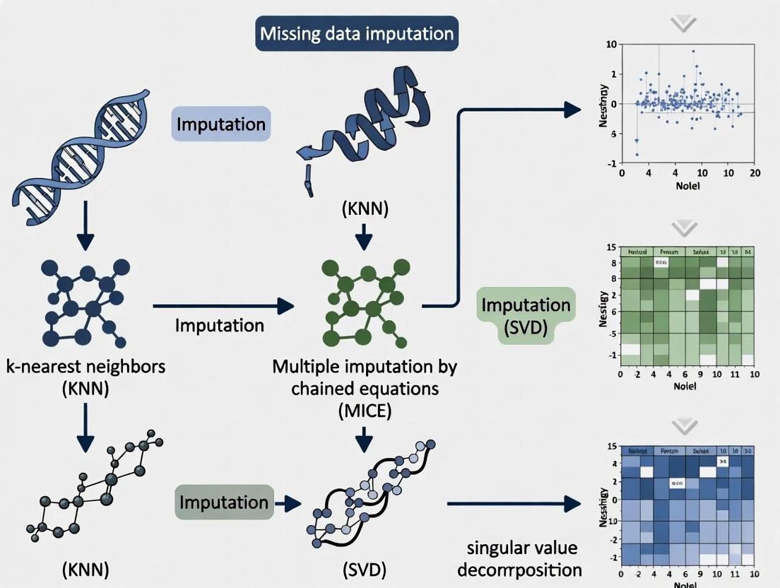
Navigating Missing Data in Omics: A Comprehensive Guide to Imputation Methods for Robust Biomedical Research
Missing data is a pervasive challenge in omics studies, threatening the validity of downstream analyses and biological discoveries.
Navigating Missing Data in Omics: A Comprehensive Guide to Imputation Methods for Robust Biomedical Research
Abstract
Missing data is a pervasive challenge in omics studies, threatening the validity of downstream analyses and biological discoveries. This article provides a comprehensive guide for researchers and drug development professionals on handling missing values in genomics, transcriptomics, proteomics, and metabolomics datasets. We explore the foundational concepts of missing data mechanisms—MCAR, MAR, and MNAR—and their implications for multi-omics integration. The guide systematically reviews traditional and AI-driven imputation methods, from k-nearest neighbors and MissForest to deep learning approaches like variational autoencoders. We offer practical strategies for method selection, troubleshooting common pitfalls, and validating imputation performance using downstream-centric criteria. Finally, we discuss emerging trends, including data multiple imputation (DMI) and privacy-preserving federated learning, providing a roadmap for implementing robust, reproducible missing data solutions in precision medicine and oncology research.
The Missing Data Challenge: Understanding the Why and How in Omics Research
The Prevalence and Impact of Missing Values in Multi-Omics Studies
Troubleshooting Guides
Guide 1: Diagnosing the Nature of Missing Data in Your Multi-Omics Dataset
A critical first step in handling missing data is diagnosing its nature and extent. Incorrect diagnosis can lead to the application of unsuitable imputation methods, biasing downstream analysis and compromising the validity of your biological conclusions.
Prerequisites: Your complete, untrimmed multi-omics dataset (e.g., as a data matrix or a SummarizedExperiment object in R).
Required Tools: Standard statistical software (e.g., R, Python) and functions for data summary.
| Step | Action | Expected Outcome & Interpretation |
|---|---|---|
| 1 | Quantify Missingness Per Sample and Per Feature | Outcome: A table or plot showing the percentage of missing values for each sample (row) and each molecular feature (column, e.g., a gene or protein).Interpretation: Identifies if missingness is concentrated in a few problematic samples/features, which might be candidates for removal, or if it is widespread. |
| 2 | Identify the Missingness Pattern | Outcome: Determination of whether data is missing sporadically (random cells in the matrix) or in a block-wise pattern (entire omics assays missing for a subset of samples).Interpretation: Block-wise missingness is common in multi-omics studies where not all assays were performed on all samples [1]. This requires specialized methods and cannot be handled by simple imputation. |
| 3 | Investigate the Missingness Mechanism | Outcome: A hypothesis on whether data is Missing Completely at Random (MCAR), Missing at Random (MAR), or Missing Not at Random (MNAR) [2] [3].Interpretation: MNAR is suspected when missingness is linked to the unobserved value itself (e.g., low-abundance proteins falling below a mass spectrometer's detection limit). This is the most challenging scenario to impute. |
Guide 2: Selecting an Appropriate Imputation Method
Choosing the right imputation method is paramount. The choice depends on your data's missingness pattern, the omics data types, and the sample size. The table below summarizes available methods.
Prerequisites: Completion of Troubleshooting Guide 1.
Required Tools: Imputation software packages (e.g., scikit-learn in Python, missForest, mice in R, or specialized tools like bwm [1]).
| Method Category | Example Methods | Best For / Use Case | Key Limitations |
|---|---|---|---|
| Conventional & Statistical | missForest, PMM, KNNimpute [4] [5] | Cross-sectional data with sporadic, low-level missingness; MCAR/MAR mechanisms. | Often fail to capture complex biological patterns; unsuitable for block-wise missingness or longitudinal data [4]. |
| Deep Learning (Generative) | Autoencoders (AE), Variational Autoencoders (VAE), Generative Adversarial Networks (GANs) [6] [7] | Large, high-dimensional datasets; capturing non-linear relationships and complex patterns within and between omics layers. | Require large sample sizes; can be computationally intensive and complex to train; risk of overfitting [7]. |
| Longitudinal & Multi-timepoint | LEOPARD [4] [8] | Multi-timepoint omics data where a full omics view is missing at one or more timepoints. Uses representation disentanglement to transfer temporal knowledge. | A novel method, requires validation for specific data types beyond the proteomics and metabolomics it was tested on. |
| Block-Wise Missing | bwm R package [1] | Datasets where entire omics blocks are missing for groups of samples. Uses a regularization and profile-based approach. | Performance may slightly decline as the percentage of missing data increases [1]. |
Guide 3: Validating Your Imputation Results
Imputation is an inference, and its accuracy must be assessed. Relying solely on quantitative metrics like Mean Squared Error (MSE) is insufficient, as low MSE does not guarantee the preservation of biologically meaningful variation [4].
Prerequisites: A dataset with a ground truth (e.g., a subset of originally observed data) and the imputed dataset.
Required Tools: Downstream analysis tools (e.g., for differential analysis, clustering, classification).
| Validation Approach | Procedure | Interpretation of Success |
|---|---|---|
| Statistical Agreement | Artificially mask some known values, impute them, and compare imputed vs. actual values using metrics like MSE or Percent Bias (PB). | A lower MSE/PB indicates better statistical accuracy. This is a basic sanity check. |
| Preservation of Biological Structure | Perform downstream analyses (e.g., differential expression, pathway enrichment, clustering) on both the original (with missingness) and imputed datasets. | The imputed data should recover known biological groups or pathways. For example, LEOPARD-imputed data achieved high agreement in detecting age-associated metabolites and predicting chronic kidney disease [4]. |
| Stability Analysis | Introduce small perturbations to the dataset or use multiple imputation to create several imputed datasets. | Robust biological findings should be consistent across the different imputed versions, indicating the imputation is not introducing spurious noise. |
Frequently Asked Questions (FAQs)
FAQ 1: Why can't I just remove samples or features with missing data?
While simple, this "complete-case analysis" is strongly discouraged. It drastically reduces sample size, wasting costly collected data and reducing statistical power [2] [1]. More critically, if data is not Missing Completely at Random (MCAR), removing samples can introduce severe bias into your analysis, leading to incorrect conclusions [2].
FAQ 2: What is the difference between "missing values" and "block-wise missing data"?
Missing values typically refer to sporadic, individual data points that are absent within an otherwise populated data matrix (e.g., a specific protein's measurement is missing for one sample). In contrast, block-wise missing data describes a scenario where entire subsets of data are absent. For example, in a study with genomics, proteomics, and metabolomics data, a group of samples might have completely missing proteomics data because that assay was not performed on them [1]. This is a common and major challenge in multi-omics integration.
FAQ 3: Are deep learning methods always superior for imputing multi-omics data?
Not always. Deep learning models (like VAEs and GANs) excel at capturing complex, non-linear relationships in large, high-dimensional datasets [6] [7]. However, they often require large sample sizes to train effectively without overfitting. For smaller studies, well-established statistical methods may be more stable and reliable. The choice should be guided by your data's scale and complexity.
FAQ 4: How do I handle missing data in a longitudinal multi-omics study?
Longitudinal data adds a temporal dimension, making the problem more complex. Generic imputation methods that learn direct mappings between views are suboptimal because they cannot capture temporal variation and may overfit to specific timepoints [4]. You need methods specifically designed for this context, such as LEOPARD, which disentangles omics data into time-invariant (content) and time-specific (temporal) representations, allowing it to transfer knowledge across timepoints to complete missing views [4] [8].
Experimental Protocols
Protocol: Missing View Completion Using the LEOPARD Framework
This protocol outlines the procedure for implementing LEOPARD (missing view completion for multi-timepoint omics data via representation disentanglement and temporal knowledge transfer), a state-of-the-art method for handling block-wise missingness in longitudinal studies [4].
Principle: LEOPARD factorizes multi-timepoint omics data into two latent representations: an omics-specific content (the intrinsic biological signal) and a timepoint-specific temporal knowledge. It then completes a missing view at a target timepoint by transferring the appropriate temporal knowledge to the available omics content.
Key Research Reagent Solutions
| Item | Function in the LEOPARD Protocol |
|---|---|
| Longitudinal Multi-omics Dataset | The input data containing multiple "views" (e.g., proteomics and metabolomics) measured at multiple timepoints. Some views are completely missing at some timepoints. |
| Content Encoder (Neural Network) | Learns to extract a view-invariant, fundamental biological representation from the input omics data. |
| Temporal Encoder (Neural Network) | Learns to extract a time-specific representation that captures the dynamics and changes across timepoints. |
| Generator with AdaIN | Reconstructs or completes omics views by applying the temporal representation (via Adaptive Instance Normalization) to the content representation. |
| Multi-task Discriminator | Guides the generator to produce imputed data that is indistinguishable from real, observed data. |
Step-by-Step Procedure
Data Preparation and Partitioning:
- Format your data into matrices for each view (e.g., V1, V2) and each timepoint (e.g., T1, T2).
- Partition the samples into training, validation, and test sets (e.g., 64%, 16%, 20% as in the original study [4]).
- Artificially mask the view-timepoint block intended for imputation in the test set (e.g., mask view V2 at time T2 for all test samples, denoted as ({{{\mathcal{D}}}}_{v={{\rm{v}}}2,t={{\rm{t}}}2}^{{{\rm{test}}}})).
Model Architecture Setup:
- Initialize Networks: Set up the content encoder, temporal encoder, generator, and discriminator neural networks.
- Define Loss Functions: Configure the composite loss function used for training LEOPARD, which includes:
- Contrastive Loss (NT-Xent): Ensures that representations from the same sample are similar and from different samples are distinct.
- Representation Loss: Encourages the disentanglement of content and temporal representations.
- Reconstruction Loss: Measures how well the generator can reconstruct the input from its representations.
- Adversarial Loss: From the discriminator, ensuring generated data is realistic.
Model Training:
- Train the model on the training set by iteratively minimizing the total loss.
- Use the validation set for early stopping to prevent overfitting.
- The model learns to factorize the data and transfer knowledge without directly seeing the missing view-timepoint combination in the training data.
Inference and Imputation:
- Feed the test samples with the missing view into the trained LEOPARD model.
- The model uses the content from an available view and the temporal knowledge from the target timepoint to generate the missing view.
Validation:
- Compare the imputed data against the held-out true values (if available) using quantitative metrics (MSE, PB).
- Perform downstream biological analysis (e.g., association studies, classification) to confirm that the imputed data retains biologically plausible signals [4].
Workflow Diagram: LEOPARD Architecture
Protocol: Handling Block-Wise Missing Data with a Profile-Based Framework
This protocol is based on the bwm R package, which provides a unified feature selection model for datasets with block-wise missingness without relying on imputation [1].
Principle: Instead of imputing missing blocks, the method groups samples into "profiles" based on which omics sources are available. It then learns a unified model across all profiles, integrating information from all available data without discarding samples.
Step-by-Step Procedure
Data Preparation:
- Organize your multi-omics data into matrices, one for each omics source (e.g., Transcriptomics, Proteomics, Metabolomics).
Profile Identification:
- For each sample, create a binary indicator vector showing the presence (1) or absence (0) of each omics source.
- Convert this binary vector into a decimal number, called the "profile." For example, in a 3-omics study, a sample with only Transcriptomics and Proteomics data would have a vector
[1, 1, 0], which corresponds to a specific profile ID. - Group all samples sharing the same profile.
Model Formulation:
- The framework learns a linear model that integrates the different omics sources. The model is defined as: ( y = \sum{i=1}^{S} \alphai Xi \betai + \epsilon ) where (Xi) is the data matrix for the (i)-th omics source, (\betai) are the feature coefficients for that source, and (\alpha_i) are profile-specific parameters that integrate the sources [1].
- The model is trained using all profiles simultaneously, allowing it to learn from all available data.
Model Fitting and Prediction:
- Use the
bwmR package to fit the model to your data for either regression or classification tasks. - The fitted model can then be used to make predictions on new data, even if the new data has a block-wise missing pattern seen in the training profiles.
- Use the
Workflow Diagram: Profile-Based Handling of Block-Missing Data
FAQ: Fundamental Concepts
Q1: What are the core types of missing data mechanisms? According to Rubin's (1976) framework, missing data mechanisms are classified into three primary types: Missing Completely at Random (MCAR), Missing at Random (MAR), and Missing Not at Random (MNAR). The key difference lies in whether the probability of a value being missing depends on the observed data, the unobserved data, or neither [9] [10].
Q2: How does the missing data mechanism affect my analysis? The mechanism dictates which statistical methods will provide valid, unbiased results. Simple methods like complete-case analysis often only work under the restrictive MCAR assumption. In contrast, modern methods like multiple imputation are valid under the broader MAR condition. Using a method inappropriate for your data's mechanism can lead to biased estimates and misleading conclusions [9] [11].
Q3: Can I statistically test to determine the missing data mechanism in my dataset? There is no definitive statistical test to distinguish between all mechanisms, particularly between MAR and MNAR [11] [12]. Determining the mechanism is not a purely statistical exercise; it requires careful consideration of the data collection process, subject-matter expertise, and reasoning about the potential causes for missingness [10] [12].
Troubleshooting Guide: Diagnosis and Handling
Problem: I need a clear, actionable workflow to classify missing data in my omics experiment. This diagnostic flowchart outlines the key questions to ask about your dataset to determine the most likely missing data mechanism.
Problem: I have identified the mechanism and need to select an appropriate imputation method. The suitable method depends on your identified missing data mechanism. The table below summarizes standard and advanced options.
| Mechanism | Recommended Methods | Key Considerations for Omics Data |
|---|---|---|
| MCAR | Complete-case analysis, Mean/Median imputation, Single imputation [9] [11] | While unbiased, complete-case analysis discards data, which can be costly if omics measurements are expensive. Simple imputation may reduce variance artificially. |
| MAR | Multiple Imputation (MICE) [11], Iterative Imputer [13], KNNImputer [14] | These multivariate methods preserve relationships between variables. Ensure your imputation model includes variables that predict missingness to satisfy the MAR assumption. |
| MNAR | Pattern-mixture models, Selection models, Sensitivity analysis [9] | These are complex and require explicit assumptions about the missingness process. Sensitivity analysis is highly recommended to test how results vary under different MNAR scenarios [9]. |
Problem: How do I implement and evaluate these methods in a robust experimental protocol? Below is a generalized workflow for evaluating imputation methods, adaptable for omics datasets.
Protocol: Evaluating Imputation Methods with Simulated Missing Data [15]
- Baseline Dataset: Begin with a high-quality, complete omics dataset. This allows you to know the true values for comparison.
- Simulate Missingness: Artificially introduce missing values under a specific mechanism (e.g., MCAR, MAR). For MAR, you can define a rule where the probability of a value being missing depends on another fully observed variable (e.g., higher missingness in protein abundance for samples with low total ion current).
- Apply Imputation: Run the selected imputation methods (from the table above) on the dataset with simulated missing values.
- Evaluate Performance: Compare the imputed values to the known true values. Common metrics include:
- Root Mean Square Error (RMSE): Measures the magnitude of imputation errors.
- Preservation of Correlation/Covariance: Assesses if the multivariate structure of the data is maintained.
- Downstream Analysis Impact: For clinical omics, evaluate how imputation affects the sensitivity, AUC, or Kappa values of a final predictive model [15].
The Scientist's Toolkit: Research Reagent Solutions
| Tool / Reagent | Function in Missing Data Imputation |
|---|---|
Scikit-learn's SimpleImputer |
A univariate imputer for basic strategies (mean, median, most_frequent) under MCAR assumptions [13]. |
Scikit-learn's IterativeImputer |
A multivariate imputer that models each feature with missing values as a function of other features, ideal for MAR data [13]. |
Scikit-learn's KNNImputer |
A multivariate imputer that estimates missing values using the mean value from the 'k'-nearest neighbors in the dataset [13] [14]. |
| Multiple Imputation by Chained Equations (MICE) | A state-of-the-art framework for creating multiple imputed datasets, accounting for uncertainty and valid under MAR [11]. |
missingno Library (Python) |
A visualization tool for understanding the patterns and extent of missingness in a data matrix prior to imputation. |
| Random Forest Imputation | A machine learning-based approach that can capture complex, non-linear relationships for imputation, often implemented within IterativeImputer [13]. |
Frequently Asked Questions (FAQs)
FAQ 1: What are the most common sources of missing data in proteomics experiments? Missing data in proteomics frequently arises from the limitations of mass spectrometry technology. Low-abundance proteins may fall below the detection threshold, leading to missing not at random (MNAR) values. Sample handling issues, such as incomplete protein digestion or precipitation, and technical variations between instrument runs (batch effects) are also major contributors [16] [17].
FAQ 2: How does missingness in transcriptomics data differ from metabolomics? In transcriptomics, missing data is often less severe due to the high sensitivity of RNA-seq but can still occur from low RNA quality, low expression levels, or library preparation artifacts. In metabolomics, missingness is more pervasive and typically MNAR, as many metabolites are present at concentrations below the detection limit of the mass spectrometer. The chemical diversity of metabolites also makes it difficult to extract and detect all compounds equally [16] [18].
FAQ 3: What is the impact of batch effects on data missingness? Batch effects themselves may not cause missing data directly, but they complicate data integration. When combining datasets from different batches, the pattern of missing values can become more complex, leading to block-wise missingness where entire omics layers are absent for some sample groups. This severely hampers the ability to apply standard batch-effect correction methods [16] [18].
FAQ 4: Are there imputation-free methods for analyzing incomplete multi-omics datasets? Yes, some advanced methods do not require imputation. The BERT (Batch-Effect Reduction Trees) framework uses a tree-based approach to integrate batches of data, propagating features with missing values through the correction steps without imputation. Other approaches use available-case analysis, creating distinct models for different data availability "profiles" to leverage all available data without filling in gaps [16] [19].
FAQ 5: What are the best practices for handling missing data in multi-omics integration? Best practices include:
- Thorough QC: Implement quality control at every stage, from sample collection to data generation, to minimize preventable missingness [17].
- Understand the Mechanism: Diagnose whether data is Missing Completely at Random (MCAR) or Missing Not at Random (MNAR), as this guides the choice of handling method [20].
- Choose Appropriate Methods: For MNAR data, consider methods like BERT that are robust to non-random missingness. For data integration with block-wise missingness, profile-based or tree-based algorithms can be more effective than simple imputation [16] [19].
- Document and Report: Keep detailed records of all processing steps, including how missing data was handled, to ensure reproducibility [17].
Troubleshooting Guides
Problem 1: Widespread Missing Data in a Single Omics Layer
- Symptoms: A high percentage of missing values for a specific data type (e.g., proteomics) across many samples.
- Investigation & Resolution:
- Audit Sample Preparation: Review protocols for sample collection, storage, and extraction specific to that omics layer. Degraded samples or improper handling are common culprits [17].
- Check Instrument Logs: Look for technical failures or calibration issues in the instrumentation (e.g., mass spectrometer) during the runs in question [17].
- Analyze Abundance: Plot the distribution of detected values. If missingness is correlated with low signal intensity, the data is likely MNAR, and you should use methods designed for this, such as a left-censored imputation model or BERT [16] [20].
Problem 2: Inability to Integrate Datasets Due to Block-Wise Missingness
- Symptoms: Failure to run integration algorithms because entire blocks of data are missing (e.g., some patient cohorts lack metabolomics data entirely).
- Investigation & Resolution:
- Profile Your Data: Map your samples to "profiles" based on which omics layers are available. This helps visualize the pattern of block-wise missingness [19].
- Use Profile-Aware Algorithms: Employ methods like the two-step algorithm for block-wise missing data, which builds models using all available data within each profile and then combines them, rather than deleting samples with incomplete data [19].
- Leverage Tree-Based Integration: Implement a framework like BERT, which is explicitly designed to handle arbitrarily incomplete omic profiles by correcting pairs of batches and propagating missing features [16].
Problem 3: Poor Model Performance After Imputation
- Symptoms: Predictive models or clustering analyses perform poorly or yield biologically implausible results after imputing missing values.
- Investigation & Resolution:
- Revisit Missingness Mechanism: Confirm your imputation method aligns with the nature of your missing data (MCAR vs. MNAR). Using a method for MCAR on MNAR data can introduce severe bias [20].
- Validate with QC Metrics: Use metrics like the Average Silhouette Width (ASW) to compare data integration quality before and after imputation. A good method should improve ASW for biological labels while reducing it for batch labels [16].
- Consider Imputation-Free Models: If imputation continues to fail, switch to models that can handle missing data natively, such as the one described in [19], or use late-integration approaches that build models on individual complete layers before combining results [18].
Quantitative Data on Data Integration Methods
The table below summarizes a performance comparison between two data integration methods, BERT and HarmonizR, as evaluated on simulated datasets with varying levels of missing values [16].
Table 1: Performance Comparison of Data Integration Methods on Simulated Data
| Metric | BERT | HarmonizR (Full Dissection) | HarmonizR (Blocking of 4 Batches) |
|---|---|---|---|
| Data Retention (with 50% missing values) | Retains all numeric values | Up to 27% data loss | Up to 88% data loss |
| Runtime | Up to 11x faster than HarmonizR | Baseline (slowest) | Faster than full dissection, but slower than BERT |
| Consideration of Covariates | Yes, accounts for severely imbalanced conditions | Not addressed in available results | Not addressed in available results |
Experimental Workflow for Handling Missing Data
The following diagram illustrates a recommended workflow for diagnosing and handling missing data in omics studies, from problem identification to solution implementation.
The Scientist's Toolkit: Research Reagent Solutions
Table 2: Essential Materials and Computational Tools for Omics Data Analysis
| Item | Function |
|---|---|
| Standard Operating Procedures (SOPs) | Detailed, validated protocols for every stage of data handling (tissue sampling, DNA/RNA extraction, sequencing) to reduce variability and improve reproducibility [17]. |
| Quality Control Software (e.g., FastQC) | Tools that generate quality metrics (Phred scores, read length distributions, GC content) to identify issues in sequencing runs or sample preparation before downstream analysis [17]. |
| Batch-Effect Correction Algorithms (e.g., BERT, ComBat) | Statistical methods to remove non-biological technical biases introduced by processing samples in different batches, times, or on different platforms [16] [18]. |
| Imputation & Integration Software (e.g., bwm R package) | Specialized packages that handle block-wise missing data and multi-class classification tasks without discarding valuable samples, crucial for incomplete multi-omics datasets [19]. |
| Laboratory Information Management System (LIMS) | Automated systems for proper sample tracking and metadata recording, which reduce human error and prevent sample mislabeling [17]. |
Frequently Asked Questions (FAQs)
1. What are the primary consequences of missing data on my statistical analysis? Missing data can lead to two major problems: a loss of statistical power due to effectively reducing your sample size, and the introduction of systematic bias in your parameter estimates if the data is not Missing Completely at Random (MCAR). This can distort effect estimates, lead to invalid conclusions, and reduce the generalizability of your findings [21] [22] [23]. The extent of the impact depends on the missing data mechanism (MCAR, MAR, or MNAR) and the proportion of data missing.
2. How does the type of missing data (MCAR, MAR, MNAR) affect my downstream biological interpretation? The mechanism of missingness directly influences how much your biological interpretation might be skewed.
- MCAR: Has the least impact on bias, though it can reduce statistical power. Biological conclusions are less likely to be systematically distorted [21] [22].
- MAR: Can introduce bias if not handled properly. However, this bias can often be accounted for using other observed variables in your dataset, allowing for valid biological inference with appropriate methods [22].
- MNAR: This is the most problematic scenario for biological interpretation. Here, the missingness is related to the unobserved value itself (e.g., low-abundance proteins missing in proteomics). This can severely bias biological conclusions, as the missing data is directly informative about the biological state. Specialized imputation methods designed for MNAR (e.g., left-censored methods) are often required [24] [25].
3. I work with multi-omics data where different samples are missing for different omics layers. Is imputation still possible? Yes, this is a common challenge in multi-omics integration. Recent advances in artificial intelligence and statistical learning have led to integration methods that can handle this specific issue. A subset of these models incorporates mechanisms for handling partially observed samples, either by using information from other omics layers to inform the imputation or by employing algorithms that can function with blocks of missing data [5] [3].
4. Which downstream analyses are most sensitive to missing value imputation? Research has shown that differential expression (DE) analysis is the most sensitive to the choice of imputation method. Gene clustering analysis shows intermediate sensitivity, while classification analysis appears to be the least sensitive. Therefore, particular care must be taken when selecting an imputation method for studies focused on identifying differentially expressed biomarkers [26].
Troubleshooting Guides
Problem: A cluster analysis after imputation reveals unexpected sample groupings.
Diagnosis: The imputation method may have introduced artificial patterns or obscured true biological signals. Some methods can distort the covariance structure of the data.
Solution:
- Verify the missing data mechanism using visualizations (e.g., heatmaps) and statistical tests like Little's MCAR test [27] [23].
- Re-impute using a method known to better preserve data structures, such as Random Forest or least squares-based methods (LLS, LSA), which were top performers in empirical evaluations [26] [28].
- Compare the cluster stability and biological coherence of the results from different imputation methods. Use the PCA stability metrics to evaluate if the overall sample structure remains consistent after imputation [25].
Problem: The list of statistically significant differentially expressed genes/ proteins changes drastically after imputation.
Diagnosis: This is a common sign that your imputation method is influencing the variance and effect size estimates in your data. This is critical because DE analysis is highly sensitive to imputation choice [26].
Solution:
- Assess the Rate of MNAR: In proteomics and metabolomics, a high rate of MNAR can cause this issue. Evaluate whether methods designed for left-censored data (e.g., QRILC, MinProb) are more appropriate [24] [25].
- Benchmark Performance: If a ground-truth dataset is available, evaluate methods based on the Normalized Root Mean Square Error (NRMSE) for protein abundance and, more importantly, the accuracy of recovering true positive differential expressions and controlling the false discovery rate [24].
- Select a Robust Method: Studies have shown that Random Forest imputation can consistently achieve a high number of true positives while maintaining a low false altered-protein discovery rate (FADR < 5%) [24].
Performance Comparison of Common Imputation Methods
The table below summarizes the performance of various imputation methods based on large-scale benchmarking studies in omics. NRMSE (Normalized Root Mean Square Error) is a common metric, where a lower value indicates better accuracy.
Table 1: Evaluation of Imputation Method Performance Across Omics Data Types
| Imputation Method | Category | Reported Performance (NRMSE & Biological Impact) | Best Suited For Data Type | Key Strengths |
|---|---|---|---|---|
| Random Forest (RF) | Machine Learning | Consistently low NRMSE; high true positives with low FADR [24] [28] | Genomics, Proteomics [28] [24] | Handles complex interactions; robust to non-linearity |
| k-Nearest Neighbors (KNN) | Local Similarity | Good performance, often second to RF; preserves data structure [28] [25] | Gene Expression, Proteomics [26] [25] | Simple; good for MCAR/MAR; works for numerical/categorical data |
| Bayesian PCA (BPCA) | Global Structure | Top performer in downstream empirical evaluation [26] | Microarray Gene Expression [26] | Effective for low-complexity data; handles global correlations |
| Least Squares Adaptive (LSA) | Local Similarity | Top performer in downstream empirical evaluation [26] | Microarray Gene Expression [26] | Adapts to local data structure; performs well in high-complexity data |
| Local Least Squares (LLS) | Local Similarity | Ranked high in proteomics workflow evaluation [25] | Gene Expression, Proteomics [26] [25] | Combines KNN with regression for improved accuracy |
| Singular Value Decomposition (SVD) | Global Structure | Performance varies; generally outperformed by BPCA and RF [26] [24] | Gene Expression [26] | Captures global trends in the data |
| Quantile Regression Imputation (QRILC) | Left-Censored | Effective for left-censored data (MNAR) [25] | Proteomics, Metabolomics [25] | Specifically designed for MNAR; preserves tail distributions |
| Mean/Median Imputation | Single Value | Poor performance; underestimates variance; not recommended for >5-10% missingness [25] [21] | Any (as a basic baseline only) | Extreme simplicity |
Experimental Protocol: Evaluating Imputation Method Performance
This protocol is adapted from a comparative study on label-free quantitative proteomics [24] and can be adapted for other omics data types.
Objective: To systematically evaluate the performance of different missing value imputation methods on a dataset where the true values are known.
Required Materials and Reagents: Table 2: Essential Research Reagent Solutions for Imputation Benchmarking
| Item Name | Function / Explanation |
|---|---|
| Benchmark Dataset | A complete, high-quality dataset with known values (e.g., spike-in proteins in a complex background) [24]. |
| Statistical Software (R/Python) | Platform for implementing and testing different imputation algorithms. |
| NAguideR Tool | An online/web tool that automates the evaluation of 23 imputation methods for proteomics data [25]. |
| NAsImpute R Package | A dedicated R package to test multiple imputation methods on a user's own genomic dataset [28]. |
Methodology:
- Start with a Complete Dataset: Begin with a high-quality dataset that has no missing values (CD). This serves as your ground truth [26] [24].
- Introduce Simulated Missing Values: Artificially generate missing values into the complete dataset under controlled conditions.
- Vary the overall missing rate (e.g., 10%, 20%, 30%).
- Vary the proportion of MNAR (e.g., 20%, 50%, 80%) to simulate different missingness mechanisms. For MNAR, typically remove low abundance values [24].
- Apply Imputation Methods: Run a suite of imputation methods (e.g., RF, KNN, BPCA, LLS, QRILC) on the datasets with simulated missing values.
- Quantitative Accuracy Assessment:
- Downstream Biological Impact Assessment:
- Perform a key downstream analysis (e.g., differential expression analysis) on both the original complete data and the imputed data.
- Compare the results by calculating:
- The number of True Positives (TPs) correctly identified.
- The False Altered-discovery Rate (FADR), which is the proportion of false positives [24].
- For pathways analysis, check if biologically relevant pathways are consistently detected after imputation [24].
Workflow and Relationship Diagrams
Imputation Evaluation Workflow
This diagram outlines the logical flow for a rigorous experimental evaluation of imputation methods.
Missing Data Impacts on Analysis
This diagram illustrates the causal relationship between the type of missing data and its consequences for statistical analysis.
The Critical Role of Imputation in Multi-Omics Data Integration
Troubleshooting Guides
Problem: After integrating multiple omics datasets, your analysis reveals unexpected biological patterns that may be artifacts of missing data rather than true biology.
Solution: Diagnose the missing data mechanism before selecting an integration method [3] [2].
- Check Missing Value Patterns: Create a missingness heatmap to visualize whether missing values cluster by sample group, omics type, or experimental batch. MNAR often shows distinct patterns where low-abundance molecules are systematically missing [25] [29].
- Mechanism-Specific Imputation: Apply methods designed for your specific missing data type. For MNAR data (common in proteomics and metabolomics), use QRILC or MinProb. For MCAR/MAR data, consider KNN, RF, or Bayesian approaches [30] [25] [29].
- Post-Imputation Validation: Use NRMSE (Normalized Root Mean Square Error) and PCA stability metrics to evaluate whether imputation preserves the original data structure without introducing artifacts [25].
Prevention: Implement study designs that minimize missing data through sufficient sample quality controls, standardized protocols, and appropriate sequencing depths or MS detection limits [17].
How to Handle Unmatched Samples Across Omics Layers?
Problem: Your dataset contains samples with complete data for some omics types but missing entire omics profiles for others, creating integration challenges.
Solution: Utilize integration methods specifically designed for unmatched samples or apply advanced imputation strategies.
- Generative Models: Implement deep learning approaches like Variational Autoencoders (VAEs) that can learn latent representations from incomplete samples and generate plausible imputations [31] [5].
- Multi-Omics Imputation: Apply methods like MOFA+ or Bayesian networks that can handle missingness at the sample level by leveraging patterns across all available omics data [32].
- Strategic Subsetting: For method validation, create a complete subset of samples to establish baseline patterns, then compare results from your imputed dataset to ensure consistency [3].
Which Imputation Method Should I Choose for My Specific Multi-Omics Study?
Problem: The overwhelming number of available imputation methods makes selecting the optimal approach challenging for your specific data type and research question.
Solution: Match imputation methods to your data characteristics and analytical goals using the decision framework below.
- Data Type Considerations: Proteomics data with abundant MNAR requires different methods (QRILC, MinProb) than transcriptomics data with mostly MCAR (KNN, RF) [25] [29].
- Sample Size Constraints: For small sample sizes (<50), prefer simpler methods like median or quantile regression. For larger datasets (>100), machine learning approaches like RF or deep learning methods become more viable [30].
- Downstream Analysis Alignment: If your goal is differential analysis, choose methods that preserve variance structure (RF, QRILC). For clustering applications, prioritize methods that maintain sample relationships (KNN, VAE) [30] [29].
Validation Protocol: Always implement multiple imputation methods and compare their impact on your downstream analyses using the evaluation metrics in Section 3.
Frequently Asked Questions (FAQs)
What Are the Main Types of Missing Data in Multi-Omics Studies?
Missing data in multi-omics studies fall into three categories based on the underlying mechanism [3] [2]:
- Missing Completely at Random (MCAR): Missingness occurs randomly with no relationship to observed or unobserved data. Example: technical failures during sequencing [2].
- Missing at Random (MAR): Missingness relates to observed variables but not the missing values themselves. Example: samples with lower overall RNA quality having more missing transcriptomic values [2].
- Missing Not at Random (MNAR): Missingness depends on the actual missing values. Example: protein abundances below mass spectrometry detection limits [25] [2].
How Much Missing Data is Too Much for Reliable Integration?
There's no universal threshold, but these guidelines apply:
- <5% missingness: Most methods perform well; simple imputation (mean, median) may suffice [25].
- 5-20% missingness: Requires more sophisticated methods (KNN, RF, SVD); careful validation needed [30].
- >20% missingness: Advanced methods essential (VAE, Bayesian networks, QRILC); results require extensive validation [30] [32].
- >30% missingness: Consider imputation-free methods or acknowledge significant limitations in interpretation [30].
Critical factors include whether missingness is balanced across sample groups and whether the mechanism is consistent across omics types [30] [3].
Can I Simply Remove Samples or Features with Missing Values?
Removing incomplete samples or features is generally discouraged in multi-omics studies because:
- Data Loss: Removing samples with any missing values across multi-omics datasets can drastically reduce sample size and statistical power [3].
- Bias Introduction: Complete-case analysis assumes data is MCAR, which is rarely true in omics studies, potentially introducing selection bias [3] [2].
- Biological Insight Loss: Removing features with missing values may eliminate biologically important molecules that are differentially present across conditions [25].
Exception: Features with >80% missingness are often removed before imputation, following the "modified 80% rule" [29].
How Do I Validate My Chosen Imputation Method?
Implement a multi-faceted validation approach:
- Statistical Metrics: Calculate NRMSE (Normalized Root Mean Square Error) for imputation accuracy and PCC (Pearson Correlation Coefficient) for relationship preservation [25].
- Structural Preservation: Use PCA to compare data structure before and after imputation, evaluating metrics like explained variance changes and sample displacement [25] [29].
- Biological Plausibility: Check whether imputation results in biologically consistent patterns rather than artifactual clusters or associations [17].
- Downstream Analysis Robustness: Test whether your primary conclusions (e.g., differential expression) remain consistent across different imputation approaches [30].
What Tools Are Available for Multi-Omics Imputation?
Table: Software Tools for Multi-Omics Data Imputation
| Tool Name | Primary Method | omics Types | Missing Data Handling | Reference |
|---|---|---|---|---|
| BayesNetty | Bayesian Networks | Multi-omics | MNAR/MAR/MCAR | [32] |
| NAguideR | 23 Method Comparison | Proteomics, Metabolomics | MNAR/MAR/MCAR | [25] |
| MetImp | Multiple Methods | Metabolomics | MNAR/MAR/MCAR | [29] |
| VIPCCA/VIMCCA | Variational Autoencoders | Single-cell multi-omics | Unpaired/Paired data | [31] |
| MOFA+ | Factor Analysis | Multi-omics | Missing entire views | [31] |
Performance Evaluation of Imputation Methods
Table: Comparative Performance of Common Imputation Methods Across Omics Types
| Method | MCAR Performance | MNAR Performance | Data Types | Computational Demand | Key Strengths | Key Limitations |
|---|---|---|---|---|---|---|
| K-Nearest Neighbors (KNN) | Good (NRMSE: 0.2-0.4) | Poor (NRMSE: >0.8) | All omics types | Moderate | Preserves local data structure | Fails with high missingness [30] |
| Random Forest (RF) | Excellent (NRMSE: 0.1-0.3) | Fair (NRMSE: 0.5-0.7) | All omics types | High | Handles complex interactions | Computationally intensive [29] |
| QRILC | Fair (NRMSE: 0.4-0.6) | Excellent (NRMSE: 0.1-0.3) | Proteomics, Metabolomics | Low | Specifically for left-censored MNAR | Assumes log-normal distribution [25] [29] |
| Bayesian PCA | Good (NRMSE: 0.2-0.4) | Good (NRMSE: 0.3-0.5) | All omics types | Moderate | Provides uncertainty estimates | Complex implementation [30] |
| Mean/Median | Fair (NRMSE: 0.4-0.6) | Poor (NRMSE: >0.8) | All omics types | Low | Simple, fast | Underestimates variance [25] |
| VAE (Deep Learning) | Excellent (NRMSE: 0.1-0.3) | Good (NRMSE: 0.3-0.5) | All omics types | Very High | Captures complex non-linear patterns | Requires large sample sizes [31] |
Experimental Protocols
Protocol 1: Evaluation Framework for Imputation Methods
Purpose: Systematically compare and validate imputation methods for your specific multi-omics dataset.
Materials:
- Multi-omics dataset with known missing value patterns
- Computing environment with sufficient RAM and processing power
- Software tools (R, Python, or specialized imputation packages)
Procedure:
- Data Preparation: Filter out features with >80% missingness across samples [29].
- Missingness Characterization: Visualize missing value patterns using heatmaps and quantify missingness per sample and per feature.
- Method Application: Apply 3-5 candidate imputation methods appropriate for your suspected missing data mechanism.
- Validation: Implement the following evaluation pipeline:
Evaluation Metrics:
- NRMSE: Calculate using known values artificially set to missing [25] [29].
- PCA Stability: Assess sample clustering consistency before and after imputation [25].
- Correlation Structure: Compare correlation patterns between complete and imputed datasets [29].
Protocol 2: Handling MNAR Data in Proteomics/Matabolomics
Purpose: Specifically address left-censored missing data common in mass spectrometry-based proteomics and metabolomics.
Materials:
- MS-based quantification data
- R environment with
imputeLCMDandNAguideRpackages [25]
Procedure:
- Data Preprocessing: Perform normalization and log-transformation of your intensity data.
- MNAR Diagnosis: Confirm left-censored mechanism by analyzing missingness vs. abundance relationships.
- QRILC Implementation:
- MinProb Alternative: Apply probabilistic minimum imputation for comparison:
- Distribution Validation: Compare distributions of imputed vs. observed values using quantile-quantile plots.
Troubleshooting: If imputation creates outliers or distorts distributions, adjust tuning parameters or consider a hybrid approach combining QRILC with KNN.
Research Reagent Solutions
Table: Essential Computational Tools for Multi-Omics Imputation
| Tool/Category | Specific Examples | Primary Function | Application Context |
|---|---|---|---|
| R Packages | imputeLCMD, missForest, VIM |
MNAR imputation, Random Forest imputation | General multi-omics imputation |
| Python Libraries | scikit-learn, Autoimpute, DataWig |
KNN, MICE, Deep learning imputation | Large-scale multi-omics data |
| Specialized Software | NAguideR, MetImp, BayesNetty |
Method comparison, Metabolomics imputation, Bayesian networks | Method selection, Targeted analysis |
| Deep Learning Frameworks | TensorFlow, PyTorch |
Variational Autoencoders, GANs | Complex multi-omics integration |
| Workflow Managers | Nextflow, Snakemake |
Pipeline reproducibility | Production-scale imputation |
Method Selection Workflow
The following diagram provides a systematic approach for selecting the appropriate imputation method based on your data characteristics and research goals:
From Simple Replacement to AI: A Practical Catalog of Imputation Techniques
Single-value imputation refers to a family of techniques where each missing value in a dataset is replaced with one specific, estimated value. This approach transforms an incomplete dataset into a complete matrix that can be analyzed using standard statistical methods. These procedures do not define an explicit model for the partially missing data but instead fill gaps using algorithms ranging from simple value substitution to more sophisticated predictive methods [33].
In omics research, including genomics, transcriptomics, proteomics, and metabolomics, missing values routinely occur due to various technical and biological factors. In mass spectrometry-based proteomics, for instance, missing values may arise from proteins existing at abundances below instrument detection limits, sample loss during preparation, or poor ionization efficiency. These missingness mechanisms are broadly categorized as Missing at Random (MAR) or Missing Not at Random (MNAR), with MNAR being particularly prevalent in proteomic data where values are missing due to abundance-dependent detection limitations [24]. Single-value replacement methods provide a practical solution to enable downstream statistical analyses that require complete datasets.
FAQ: Understanding Single-Value Replacement
1. What is the fundamental difference between single and multiple imputation?
Single imputation fills each missing value with one specific estimate, creating a single complete dataset that can be analyzed with standard methods. However, it does not account for the uncertainty inherent in the estimation process. In contrast, multiple imputation generates several different plausible values for each missing data point, creating multiple complete datasets. Analyses are performed across all datasets, and results are pooled, providing standard errors that reflect both sampling variability and uncertainty about the missing values [33].
2. When is single-value replacement most appropriate for omics data?
Single-value replacement is particularly suitable when:
- The proportion of missing data is relatively low (e.g., <10-20%)
- The analysis method requires a complete data matrix and is robust to minor estimation errors
- Computational efficiency is a priority for large-scale datasets
- The data structure suggests a clear imputation model (e.g., MNAR mechanisms in proteomics where left-censored methods are appropriate) [24] [33]
3. What are the primary limitations of single-value replacement methods?
The main limitations include:
- Distortion of variance: Treated as actual observations, imputed values don't reflect estimation uncertainty
- Biased estimates: Variances and covariances are often biased toward zero when using mean imputation
- Distorted data structure: The filled-in values may not preserve the original joint distribution of variables
- Risk of artifactual findings: Spurious patterns may be introduced if the imputation model is inappropriate [33]
4. How does the missingness mechanism (MNAR vs. MAR) affect method selection?
The missingness mechanism significantly impacts method performance:
- For MNAR data (common in proteomics), left-censored methods like LOD or random drawing from a left-censored normal distribution are often appropriate as they replace missing values with small values near the detection limit
- For MAR data, methods that leverage correlations between variables (e.g., kNN, regression imputation) typically perform better as they use observed data to predict missing values [24]
5. What validation approaches are recommended after imputation?
Performance validation should include:
- Assessing impact on downstream analyses (e.g., differential expression results)
- Comparing known spike-in values with imputed values when available
- Evaluating the preservation of biological signatures and pathways
- Using normalized root mean square error (NRMSE) to quantify imputation accuracy when true values are known [24]
Troubleshooting Common Experimental Issues
Problem: Distorted Variance After Imputation
Issue: After applying single-value replacement, variance estimates and covariances are biased toward zero, affecting downstream statistical tests.
Solution: Apply statistical adjustments to correct for bias:
- For unconditional mean imputation, multiply the sample variance from filled-in data by (n-1)/(n(j)-1), where n is total sample size and n(j) is the number of observed values for variable j [33]
- Consider stochastic regression imputation instead of deterministic methods, as it preserves more natural variability by adding random noise to predictions [33]
Prevention: Use methods that preserve data structure better, such as stochastic regression imputation or maximum likelihood approaches, particularly when variance estimation is critical to your analysis.
Problem: Poor Performance with High Missingness Rates
Issue: When missing value rates exceed 20-30%, single-value replacement methods produce unreliable estimates and distort data structure.
Solution:
- Consider multiple imputation methods for high missingness rates (>20%)
- Implement methods specifically designed for high missingness scenarios in omics data (e.g., random forest-based imputation)
- Evaluate whether the analysis can be restricted to features with lower missingness rates [24]
Prevention: Optimize experimental design to minimize missing values through technical replicates, adequate sample quality control, and using platforms with demonstrated low missing value rates.
Problem: Inconsistent Biological Results After Imputation
Issue: Downstream analyses (pathway analysis, clustering) yield different biological interpretations depending on the imputation method used.
Solution:
- Compare multiple imputation methods using validation metrics when possible
- Apply method consistency checks using known biological positives (e.g., spike-in proteins, established pathway alterations)
- Use ensemble approaches or select methods that demonstrate better performance in benchmarking studies for your data type [24]
Prevention: Document and report the imputation method and parameters as part of your analysis pipeline to ensure reproducibility.
Performance Comparison of Single-Value Replacement Methods
Table 1: Comparison of single-value imputation methods for omics data
| Method | Mechanism | Pros | Cons | Best For |
|---|---|---|---|---|
| Unconditional Mean | Replaces with column mean | Simple, preserves mean | Severely underestimates variance, distorts distributions | Initial data exploration only [33] |
| k-Nearest Neighbors (kNN) | Uses similar samples/features | Captures local structure, handles MAR | Sensitive to k choice, computational cost for large datasets [24] | Gene expression data with moderate missingness [5] |
| Left-Censored (LOD, ND) | Replaces with low values near detection limit | Biologically plausible for MNAR | May introduce bias if MNAR assumption incorrect [24] | Proteomics data with abundance-dependent missingness [24] |
| Regression Imputation | Predicts using observed variables | Uses correlation structure, efficient | Overfits with many variables, inflates correlations [33] | Datasets with strong variable correlations |
| Random Forest (RF) | Machine learning prediction | Handles complex interactions, robust | Computationally intensive, complex implementation [24] | Various omics data, shown to outperform other methods [24] |
| Stochastic Regression | Regression with added random noise | Preserves variance better than deterministic | Requires appropriate error distribution specification [33] | When variance preservation is important |
Table 2: Performance metrics of imputation methods from proteomics benchmarking study [24]
| Method | NRMSE (20% MNAR) | NRMSE (50% MNAR) | NRMSE (80% MNAR) | True Positives | False Discovery Rate |
|---|---|---|---|---|---|
| Random Forest | Lowest | Lowest | Lowest | High | <5% |
| kNN | Intermediate | Intermediate | Intermediate | Medium | 5-15% |
| LOD | Higher | Higher | Lower | Low | Variable |
| SVD | Intermediate | Intermediate | Higher | Medium | 5-15% |
Experimental Protocols for Method Evaluation
Benchmarking Protocol for Imputation Methods
Objective: Systematically evaluate the performance of single-value replacement methods using a ground-truth dataset.
Materials:
- Complete omics dataset with known values (e.g., spike-in proteins in proteomics)
- Computing environment with imputation algorithms implemented
Procedure:
- Data Preparation: Start with a complete dataset (no missing values) where true values are known
- Missing Value Introduction: Artificially introduce missing values with specified rates (e.g., 10%, 20%, 30%) and MNAR mechanisms (e.g., 20%, 50%, 80% MNAR)
- Method Application: Apply each imputation method to the dataset with introduced missingness
- Performance Calculation:
- Compute Normalized Root Mean Square Error (NRMSE) between imputed and true values
- Compare protein ratios between groups after imputation
- Calculate true positives and false discovery rates for differential expression analysis
- Biological Validation: Assess whether relevant biological pathways are detected after imputation [24]
Expected Outcomes: Quantitative metrics enabling objective comparison of method accuracy and impact on downstream analyses.
Parameter Optimization Protocol
Objective: Determine optimal parameters for each imputation method to maximize performance.
Materials: Dataset with representative missingness patterns for your omics platform
Procedure:
- kNN: Test k-values (number of neighbors) from 5-20, select value minimizing NRMSE
- SVD/BPCA: Test number of principal components (1-10), select optimal based on NRMSE
- Random Forest: Test number of trees (50-500), though method is generally robust to this parameter [24]
- Validation: Use cross-validation or holdout dataset to prevent overfitting
Expected Outcomes: Method-specific parameter settings optimized for your data type and missingness patterns.
Workflow Visualization
Imputation Method Evaluation Workflow
Research Reagent Solutions
Table 3: Key platforms and reagents for single-cell omics studies involving missing data
| Platform/Reagent | Function | Application Context | Considerations |
|---|---|---|---|
| 10X Genomics Chromium | High-throughput scRNA-seq | Large-scale single-cell studies | Higher multiplet rates, requires high cell input [34] |
| BD Rhapsody | Microwell-based single-cell analysis | Targeted transcriptomics | Lower recovery rates, fixed panel design [34] |
| cellenONE | Image-based single-cell dispenser | Rare cell analysis, high accuracy | Lower throughput but superior cell selection [34] |
| IonStar MS Workflow | Label-free quantitative proteomics | Proteomics with low missing values | High-quality data for benchmarking [24] |
| CITE-seq/REAP-seq | Multimodal protein and RNA measurement | Cellular indexing of transcriptomes and epitopes | Limited by antibody availability [35] |
| SPLIT-seq | Low-cost scRNA-seq method | Cost-effective large-scale studies | Higher technical noise and missing values |
Core Concepts: kNN Imputation
What is kNN imputation and how does it work?
k-Nearest Neighbors (kNN) imputation is a data preprocessing technique used to fill missing values by leveraging the similarity between data points [36]. It operates on a simple principle: for any sample with a missing value, find the 'k' most similar samples (neighbors) in the dataset that have the value present, and use their values to estimate the missing one [37] [38].
The process involves three key steps [37]:
- Identifying Missing Values: The algorithm first locates all missing values (typically encoded as NaN) in the dataset.
- Finding Nearest Neighbors: For each data point with a missing value, it calculates distances to all other samples using a specified distance metric (like Euclidean distance), considering only the features where both points have observed values.
- Imputing Missing Values: The missing value is then imputed using the mean (for continuous data) or mode (for categorical data) of the corresponding values from the k-nearest neighbors.
What are the advantages of kNN imputation over simpler methods for omics data?
kNN imputation offers several advantages that make it particularly valuable for omics data analysis [36] [38]:
- Preserves Data Relationships: Unlike mean/median imputation which can distort variance and relationships, kNN retains the local structure and correlations within the dataset, which is crucial for maintaining biological signals in omics data.
- Non-Parametric: kNN does not make strong assumptions about data distribution, providing flexibility for various omics data types that may not follow standard distributions.
- Handles Multivariate Patterns: Uses multiple features simultaneously to predict missing values, capturing complex biological relationships that univariate methods miss.
- Adapts to Local Patterns: By finding similar samples, it can accommodate subgroup-specific patterns that might exist in heterogeneous omics datasets.
What are the main limitations of kNN imputation in omics research?
Despite its advantages, kNN imputation has several limitations that researchers should consider [36] [38]:
- Computational Intensity: The algorithm requires calculating pairwise distances between all samples, which becomes computationally expensive for large omics datasets with thousands of samples.
- Sensitivity to Data Sparsity: Struggles when too many missing values exist, as there may not be enough complete cases to find reliable neighbors.
- Dependence on Parameter Tuning: Performance heavily depends on appropriate selection of k (number of neighbors) and the distance metric.
- Requires Complete Features for Neighbors: Cannot impute values when all samples have missing values for a particular feature.
- Assumes Similarity Implies Similar Values: May perform poorly when the missingness mechanism is non-random (NMAR) and related to the missing values themselves.
Implementation and Experimental Protocols
How do I implement basic kNN imputation in Python?
Here's a basic implementation using scikit-learn's KNNImputer [37] [14]:
What is the detailed experimental protocol for kNN imputation in omics studies?
A robust experimental protocol for kNN imputation in omics research should include these key steps [37] [36]:
Data Preprocessing:
- Standardize/normalize numerical features to ensure equal weighting in distance calculations
- Encode categorical variables numerically if present
- Identify and document missing value patterns
Parameter Optimization:
- Use cross-validation to determine optimal k (typically 3-10)
- Test different distance metrics (Euclidean, Manhattan, cosine)
- Evaluate weighting schemes (uniform vs. distance-based)
Model Training and Validation:
- Split data into training and validation sets
- For validation, artificially introduce missing values into complete cases
- Compare imputed values to ground truth using appropriate metrics
Downstream Analysis:
- Assess impact on downstream analyses (differential expression, clustering)
- Compare with alternative imputation methods
- Perform sensitivity analysis to evaluate robustness
How can I handle mixed data types (numerical and categorical) with kNN imputation?
Handling mixed data types requires preprocessing to make categorical variables compatible with kNN distance calculations [37]:
Troubleshooting Common Issues
Why is my kNN imputation producing poor results, and how can I improve them?
Poor kNN imputation performance can stem from several sources. Here are common issues and solutions [36] [38]:
Problem: Suboptimal choice of k
- Solution: Use cross-validation to find the optimal k. Start with k=3-5 and test increasing values. Smaller k captures local structure but may be noisy; larger k provides smoothing but may overlook important local patterns.
Problem: Improper feature scaling
- Solution: Always standardize (z-score normalize) or normalize (scale to [0,1]) numerical features before imputation to prevent features with larger scales from dominating distance calculations.
Problem: High percentage of missing data
- Solution: kNN works best with ≤30% missingness. For higher percentages, consider alternative methods or use rowmaxmissing parameter to exclude samples with excessive missing values.
Problem: Inappropriate distance metric
- Solution: Test different metrics: Euclidean (standard), Manhattan (more robust to outliers), or cosine similarity (for high-dimensional data).
How do I assess whether kNN imputation is working correctly for my omics data?
Use these validation strategies to evaluate kNN imputation quality [36]:
Statistical Consistency Checks:
- Compare distributions before and after imputation using histograms and Q-Q plots
- Check that imputed values fall within biologically plausible ranges
- Verify that correlation structures between variables are preserved
Validation Using Artificial Missingness:
- Artifically remove known values (5-10%) from complete cases
- Impute these artificial missing values and compare to actual values
- Calculate RMSE, MAE, or other accuracy metrics
Downstream Task Performance:
- Compare performance of classification or clustering models using imputed vs. complete-case data
- Assess whether biological conclusions remain consistent
Comparison with Alternative Methods:
- Benchmark against mean/median imputation, MICE, or other methods
- Evaluate if kNN provides substantive improvement for your specific analysis
Why is kNN imputation so slow with my large omics dataset, and how can I speed it up?
kNN imputation has computational complexity that scales quadratically with sample size, making it slow for large datasets. Consider these optimizations [36] [38]:
Algorithmic Optimizations:
- Reduce dataset dimensionality using PCA or feature selection before imputation
- Use approximate nearest neighbor algorithms instead of exact search
- Implement data sampling techniques for parameter tuning
Implementation Strategies:
- Set
copy=Falsein KNNImputer for in-place operations to reduce memory usage - Use efficient data structures and sparse matrix representations where possible
- Leverage GPU acceleration if available
- Set
Practical Workarounds:
- For very large datasets, consider alternative methods like Random Forest imputation
- Process data in batches or subsets when feasible
- Use the
col_max_missingparameter to exclude features with excessive missingness
Performance and Benchmarking
How does kNN imputation performance compare across different missingness mechanisms?
Recent benchmarking studies reveal important performance patterns across missing data mechanisms [39]:
Table 1: kNN Imputation Performance Across Missingness Mechanisms
| Mechanism | Description | kNN Performance | Considerations for Omics Data |
|---|---|---|---|
| MCAR (Missing Completely at Random) | Missingness independent of any variables | Best performance | Works well for technical missingness in omics |
| MAR (Missing at Random) | Missingness depends on observed variables | Good performance | Common in omics; requires relevant variables are observed |
| MNAR (Not Missing at Random) | Missingness depends on unobserved factors or the value itself | Poorest performance | Problematic for biological missingness (e.g., low-abundance molecules) |
How does kNN imputation compare to other methods for omics data?
Table 2: Method Comparison for Omics Data Imputation
| Method | Strengths | Limitations | Best Suited for Omics Use Cases |
|---|---|---|---|
| kNN Imputation | Preserves local structure, non-parametric, intuitive | Computationally intensive, sensitive to k choice, struggles with high missingness | Medium-sized datasets (<10,000 samples), when biological subgroups exist |
| Mean/Median Imputation | Simple, fast | Distorts distributions, underestimates variance, biases downstream analysis | Not recommended except for quick exploratory analysis |
| MICE (Multiple Imputation by Chained Equations) | Accounts for uncertainty, flexible model specification | Complex implementation, computationally intensive, difficult with high dimensions | When uncertainty quantification is crucial, smaller datasets with complex relationships |
| Matrix Factorization | Handles high sparsity, captures global patterns | Requires tuning of rank parameter, may oversmooth local patterns | Very large datasets, collaborative filtering scenarios |
| Deep Learning Methods (Autoencoders, VAEs, GANs) | Captures complex non-linear relationships, handles high-dimensional patterns | Complex implementation, requires large datasets, computationally intensive | Large-scale multi-omics integration, complex biological patterns |
Research Reagent Solutions
Table 3: Essential Tools for kNN Imputation in Omics Research
| Tool/Resource | Function | Implementation Notes |
|---|---|---|
| scikit-learn KNNImputer | Primary implementation of kNN imputation | Native in scikit-learn ≥0.22; most accessible and well-documented option [37] [14] |
| missingpy | Alternative implementation with additional features | Supports both kNN and MissForest (Random Forest imputation) [40] |
| fancyimpute | Comprehensive imputation package | Multiple advanced algorithms but may have compatibility issues with newer Python versions [41] |
| Scikit-learn preprocessing tools (StandardScaler, OrdinalEncoder) | Data preprocessing for kNN | Essential for normalizing features and encoding categorical variables [37] |
| PCA and feature selection tools | Dimensionality reduction | Critical for improving performance with high-dimensional omics data [36] |
Workflow and Algorithm Visualization
kNN Imputation Workflow
kNN Parameter Relationships
Frequently Asked Questions
What are global structure methods, and why are they used for imputation? Global structure methods, such as SVD, leverage the overall correlation structure of the entire dataset to estimate missing values. Unlike methods that only use similar rows or columns, they can provide more accurate imputation for datasets where many variables are interrelated, which is common in omics data [42].
My data has values Missing Not at Random (MNAR). Can I still use SVD? Yes. While it was once thought model-based methods were only for MAR data, studies show that SVD and other matrix factorization methods can effectively model both MAR and MNAR missingness by identifying underlying patterns in the data [42].
How do I choose the rank (number of components) for SVD imputation? The choice of rank (
k) is a trade-off between capturing signal and avoiding noise. A common method is to examine the scree plot of singular values and choosekwhere the values plateau. You can also use theirlbapackage in R for fast computation of a partial SVD, which is efficient for large omics matrices [42] [43].Should I impute before or after normalizing my data? The sequence can impact results. Some research suggests imputation of normalized data might be beneficial, but this is often context-dependent. A systematic, benchmarking analysis on your specific data type is recommended to determine the optimal workflow [42].
What are the main advantages of SVD over other imputation methods? SVD provides an optimal low-rank approximation of your data, effectively denoising while imputing. It is also a highly robust and scalable algorithm, offering a good balance of accuracy and computational speed, especially for large datasets where methods like Random Forest (RF) become very slow [42] [43].
Is there a method related to SVD that can handle missing data iteratively? Yes, the Non-linear Iterative Partial Least Squares (NIPALS) algorithm is a classical method that can compute the principal components of a dataset with missing values, thereby enabling an SVD-like decomposition and imputation without requiring a complete matrix to start.
Troubleshooting Guides
Problem: SVD Algorithm Fails on Incomplete Matrix
- Symptoms: Your software returns an error such as "Matrix contains NA/NaN/Inf" or "SVD does not support missing values."
Background: Standard SVD implementations in libraries (e.g., NumPy, base R) require a complete numeric matrix. Your omics data matrix contains missing values, which must be handled before the decomposition.
Solution 1: Use an SVD-based imputation algorithm
- Concept: These methods iteratively perform SVD while updating the missing values, converging to a complete matrix.
- Protocol:
- Initialization: Replace all missing values with initial estimates (e.g., column means).
- Decomposition: Perform a low-rank SVD on the current complete matrix.
- Reconstruction: Reconstruct the matrix using the top
kcomponents: ( X{\text{reconstructed}} = Uk \Sigmak Vk^T ). - Imputation: Replace the previously missing values in your original matrix with the corresponding values from ( X_{\text{reconstructed}} ).
- Iteration: Repeat steps 2-4 until the values in the missing positions converge (i.e., the change between iterations falls below a set tolerance).
Solution 2: Use a dedicated software function
- Concept: Many bioinformatics packages have built-in functions that implement the iterative SVD process.
- Protocol:
- In R, you can use the
impute.svd()function from thebcvpackage or thepcaMethodssuite [42]. - In Python, the
fancyimputelibrary provides anIterativeSVDcompleter.
- In R, you can use the
Problem: Poor Imputation Accuracy After SVD
- Symptoms: After imputation, downstream analyses (e.g., clustering, differential expression) yield poor or nonsensical results.
Background: Accuracy can be compromised by an incorrect number of components, the nature of the missing data, or the data's scaling.
Solution 1: Optimize the number of components (
k)- Protocol:
- Artificially introduce missing values into a complete subset of your data (e.g., 10%) where the true values are known. This is a "holdout" test.
- Run the SVD imputation algorithm with different values of
k. - For each
k, calculate the error (e.g., Root Mean Square Error) between the imputed and the known true values for the holdout set. - Select the
kthat minimizes this error.
- Protocol:
Solution 2: Re-evaluate the missing data mechanism
- Protocol:
- Assess Missingness Pattern: Plot the missing value heatmap and the distribution of missingness against intensity (log2) [42]. A concentration of missing values at low intensities suggests MNAR.
- Choose Method Accordingly: If MNAR is dominant, consider combining SVD with a method tailored for left-censored data, or ensure your SVD implementation is robust to such patterns, as some studies indicate it can be effective [42].
- Protocol:
Solution 3: Check data pre-processing
- Protocol: Ensure the data is properly transformed and normalized before imputation, as the performance of SVD can be sensitive to the data distribution [42].
Problem: SVD is Computationally Slow on Large Omics Dataset
- Symptoms: The imputation process takes an extremely long time or runs out of memory.
Background: The computational complexity of a full SVD is high for large matrices (e.g., thousands of genes and samples).
Solution 1: Use a partial SVD
- Concept: Instead of computing all components, calculate only the top
kthat explain most of the variance. - Protocol:
- In R, use the
irlba()function for fast partial SVD [42]. - In Python, use
scipy.sparse.linalg.svds.
- In R, use the
- Concept: Instead of computing all components, calculate only the top
Solution 2: Improve the algorithm implementation
- Concept: Some SVD implementations are more optimized than others.
- Protocol: Benchmark different packages. For instance, the
bigomics/playbasesource code offers a modifiedsvdImpute2()function reported to be 40% faster than the originalpcaMethodsimplementation [42].
Experimental Protocols & Data
Protocol: Benchmarking Imputation Methods Using a Holdout Set
Purpose: To empirically evaluate and compare the accuracy of different imputation methods (e.g., SVD, KNN, BPCA) on your specific omics dataset.
- Preparation: Start with a complete or nearly complete dataset (X_original).
- Introduction of Missing Values: Randomly remove a known percentage (e.g., 10-20%) of values from Xoriginal to create an incomplete matrix (Xincomplete). Keep a record of the removed values and their positions (Mask_matrix).
- Imputation: Apply each imputation method (SVD, KNN, etc.) to Xincomplete to generate an imputed matrix (Ximputed).
- Accuracy Calculation: For each method, calculate the error between the imputed values and the original values in the holdout set. Common metrics include:
- Root Mean Square Error (RMSE): Measures the magnitude of the average error.
- Mean Absolute Error (MAE): Less sensitive to large outliers than RMSE.
- Comparison: The method with the lowest error metrics is considered the most accurate for your dataset under the tested conditions.
Quantitative Comparison of Common Imputation Methods
The table below summarizes key characteristics of various imputation methods based on performance studies, particularly in proteomics [42].
| Method | Typical Use Case | Key Advantage | Key Disadvantage | Reported Accuracy Rank |
|---|---|---|---|---|
| SVD / BPCA | MAR & MNAR | Best balance of accuracy & speed; robust [42] | May require parameter tuning (rank) | Often top-ranking [42] |
| Random Forest | MAR | High accuracy [42] | Very slow for large datasets [42] | Often top-ranking [42] |
| K-Nearest Neighbors | MAR | Simple, intuitive | Performance drops with high missingness | Ranked highly in some studies [42] |
| LLS | MAR | High accuracy [42] | Can be unstable with small matrices [42] | Top-performing [42] |
| MinDet / MinProb | MNAR | Very fast [42] | Low accuracy; simple assumption [42] | Lower accuracy [42] |
The Scientist's Toolkit
| Research Reagent / Resource | Function in Imputation Analysis |
|---|---|
| R Statistical Environment | Primary platform for statistical computing and implementing imputation algorithms. |
| pcaMethods R Package | Provides multiple SVD and PCA-based imputation methods (BPCA, SVD). |
| NAguideR R Package | Evaluates and performs 23 imputation methods, facilitating benchmarking. |
| Python with Scikit-learn & SciPy | Alternative platform for matrix factorization and scientific computing. |
| irlba R Package | Computes fast, partial SVDs for large-scale datasets. |
| Complete Omics Dataset Subset | A subset of your data with no missing values, essential for creating holdout tests to validate imputation accuracy. |
Workflow and Relationship Visualizations
Imputation Method Selection Workflow
Iterative SVD Imputation Process
Missing data presents a significant challenge in omics research, where high-dimensional datasets from genomics, transcriptomics, proteomics, and metabolomics frequently contain gaps due to technical limitations, measurement errors, or quality control issues. Random Forest-based imputation methods have emerged as powerful solutions that handle the complex interactions, non-linearity, and mixed data types characteristic of omics data. This technical support center provides researchers, scientists, and drug development professionals with practical guidance for implementing MissForest and related Random Forest imputation techniques in their omics research pipelines.
Algorithm Fundamentals and Performance
How MissForest Works
MissForest is an iterative imputation technique that operates by training Random Forest models to predict each variable with missing values using all other variables as predictors [44] [45]. The algorithm follows this workflow:
- Initialization: Missing values are filled using simple imputation methods (mean for continuous variables, mode for categorical variables) [45] [46]
- Iterative Imputation: For each variable with missing values:
- The variable is treated as the response
- Observed values form the training set
- A Random Forest model predicts missing values
- Convergence Check: The process repeats until the difference between current and previous imputations stops improving or a maximum iteration limit is reached [45]
The following diagram illustrates this iterative process:
Performance Characteristics
Random Forest imputation methods demonstrate particular strengths with omics data due to their ability to handle high-dimensional settings and capture complex relationships [47]. Research shows MissForest performs well under moderate to high missingness conditions and remains robust even when data is missing not at random (NMAR) in certain cases [47].
Table 1: Performance Comparison of Imputation Methods
| Method | Data Type Handling | Non-linearity & Interactions | Computational Efficiency | Best Use Cases |
|---|---|---|---|---|
| MissForest | Mixed (continuous & categorical) | Excellent handling | Moderate to high | High-dimensional omics with complex relationships |
| KNN Imputation | Numerical (requires transformation) | Limited handling | Low with large datasets | Smaller datasets with MCAR mechanism |
| MICE with PMM | Primarily continuous | Moderate handling | High | Traditional statistical analysis |
| Mean/Median Imputation | Numerical only | No handling | Very high | Baseline reference only |
| Deep Learning Methods | Mixed types | Excellent handling | Very high computational demand | Very large omics datasets with complex patterns [7] |
Troubleshooting Guides
FAQ 1: How Do I Handle Convergence Issues?
Problem: MissForest iterations not converging or exceeding maximum iteration limit.
Solutions:
- Adjust Stopping Criteria: Modify the tolerance parameter to allow for earlier stopping when improvements become negligible
- Increase Maximum Iterations: Default is typically 10 iterations, but complex omics datasets may require more [45]
- Check Data Patterns: Investigate if specific variables with high missingness prevent convergence; consider additional preprocessing
- Alternative Initialization: Use more sophisticated initialization methods (e.g., k-nearest neighbors) instead of mean/mode
Diagnostic Script:
FAQ 2: Why Am I Getting Biased Results with Skewed Omics Data?
Problem: MissForest can produce biased estimates for highly skewed variables, common in omics data like gene expression counts [45].
Solutions:
- Data Transformation: Apply appropriate transformations (log, VST) to highly skewed variables before imputation
- Alternative Methods: Consider MICE-based Random Forest imputation (CALIBERrfimpute) for skewed data [45]
- Model Specification: Ensure proper tuning parameters (number of trees, mtry) are optimized for your specific data distribution
- Post-imputation Validation: Compare distribution of imputed values against observed values for consistency
Implementation Example:
FAQ 3: How to Manage Computational Demands with Large Omics Datasets?
Problem: MissForest becomes computationally expensive with high-dimensional omics data.
Solutions:
- Variable Selection: Pre-filter variables using variance-based or relevance-based selection
- Parallel Processing: Utilize the built-in parallelization in packages like randomForestSRC [47]
- Approximate Methods: Implement multivariate missForest (mForest) that groups variables to reduce computational load [47]
- Hardware Optimization: Use high-performance computing environments with sufficient RAM
- Alternative Packages: Explore missForestPredict for optimized prediction settings [44]
Code Optimization Example:
FAQ 4: How to Handle Mixed Data Types in Multi-omics Studies?
Problem: Integration of continuous (expression levels), categorical (mutation status), and ordinal (clinical scores) data types.
Solutions:
- Type Specification: Explicitly define variable types in function calls to ensure proper splitting rules
- Custom Initialization: Implement type-specific initialization (median for continuous, mode for categorical)
- Validation by Type: Assess imputation accuracy separately for each data type
- Package Selection: Use MissForest or missForestPredict which natively support mixed data types [44] [46]
Implementation:
Experimental Protocols and Validation
Benchmarking Protocol for Imputation Methods
When evaluating Random Forest imputation methods for omics data, follow this structured protocol:
Data Preparation:
- Start with a complete omics dataset (or create one by removing potentially problematic variables)
- Document key dataset characteristics: sample size, number of features, correlation structure
Missingness Introduction:
- Systematically introduce missing values under different mechanisms (MCAR, MAR, MNAR)
- Vary missingness proportions (5%, 10%, 20%, 30%) to assess robustness [39]
Method Implementation:
- Apply MissForest with appropriate parameter tuning
- Compare against baseline methods (mean/mode, KNN) and advanced alternatives (MICE, deep learning)
- Use consistent initialization across methods
Performance Evaluation:
- Calculate normalized root mean square error (NRMSE) for continuous variables
- Compute proportion of falsely classified (PFC) for categorical variables
- Assess downstream analysis impact (e.g., clustering stability, classification accuracy)
Table 2: Key Parameters for Random Forest Imputation
| Parameter | Recommended Setting | Adjustment Guidance | Impact on Performance |
|---|---|---|---|
| Number of Trees (ntree) | 100-500 | Increase for complex patterns | Higher values improve stability but increase computation time |
| Variables per Split (mtry) | sqrt(p) for classification, p/3 for regression | Adjust based on feature correlation | Affects model diversity and performance |
| Maximum Iterations | 10-20 | Increase if convergence is slow | Too low may stop before convergence; too high wastes computation |
| Node Size | 1 for classification, 5 for regression | Increase for noisy data | Smaller nodes capture more complex patterns but may overfit |
Validation Framework
After imputation, implement this comprehensive validation strategy:
Distribution Preservation:
- Compare distributions of observed vs. imputed values using QQ-plots and Kolmogorov-Smirnov tests
- Assess variance inflation or deflation in imputed variables
Relationship Preservation:
- Evaluate correlation structure maintenance in original vs. imputed data
- Check if biological known relationships are preserved post-imputation
Downstream Analysis Stability:
- Test robustness of differential expression results
- Evaluate clustering consistency and biomarker discovery stability
Validation Script Example:
The Scientist's Toolkit
Table 3: Essential Tools for Random Forest Imputation in Omics Research
| Tool/Resource | Type | Function | Implementation Notes |
|---|---|---|---|
| missForest R Package | Software | Primary MissForest implementation | Most straightforward implementation; limited for new data imputation |
| missForestPredict | Software | Extended MissForest for prediction settings | Supports imputation of new observations; saves models for reuse [44] |
| randomForestSRC | Software | Comprehensive Random Forest package | Includes advanced imputation methods; supports parallel processing [47] |
| miceforest (Python) | Software | Python implementation of MICE with LightGBM | Good alternative for Python workflows; handles large datasets efficiently [46] |
| High-Performance Computing Cluster | Infrastructure | Parallel processing resource | Essential for genome-scale datasets; reduces computation time from days to hours |
| Multi-omics Data Integration Framework | Methodology | Protocol for combining different data types | Critical for integrated analysis of genomics, transcriptomics, proteomics data |
Advanced Applications and Future Directions
Multi-omics Data Integration
Random Forest imputation methods show particular promise for multi-omics data integration, where missingness patterns often vary across different data layers. The capability to handle mixed data types makes MissForest suitable for integrating continuous (gene expression), binary (mutation status), and categorical (pathway membership) data in drug development pipelines.
Emerging Methodologies
Recent advances in deep learning imputation methods, including autoencoders and generative adversarial networks (GANs), offer alternatives for specific omics applications [7]. While these methods can capture complex patterns in large datasets, they typically require more computational resources and larger sample sizes than Random Forest approaches.
The development of hybrid methods that combine the robustness of Random Forests with the pattern recognition capabilities of deep learning represents a promising research direction for handling missing data in large-scale omics studies for drug discovery.
MissForest and Random Forest imputation methods provide powerful, robust solutions for handling missing data in omics research. Their ability to manage mixed data types, capture complex interactions, and scale to high-dimensional settings makes them particularly valuable for biomedical researchers and drug development professionals. By implementing the troubleshooting guides, experimental protocols, and validation frameworks provided in this technical support center, researchers can effectively address missing data challenges while maintaining the integrity of their biological findings.
FAQs: Core Concepts and Applications
Q1: How do Autoencoders (AEs) and Variational Autoencoders (VAEs) differ in their approach to learning data representations?
Both AEs and VAEs are neural networks designed to learn efficient data codings, but they fundamentally differ in how they structure their latent (hidden) space. A standard autoencoder compresses an input into a fixed-size vector in the latent space and then reconstructs the output from this vector. The primary goal is often to minimize the reconstruction error. In contrast, a Variational Autoencoder (VAE) introduces a probabilistic twist. Instead of outputting a single vector, the VAE's encoder produces the parameters of a probability distribution (typically the mean and variance of a Gaussian distribution). A random sample is then drawn from this distribution and fed to the decoder. This forces the latent space to be continuous and structured, meaning that small changes in the latent space result in small changes in the decoded output. This property makes VAEs excellent for generating new data samples, whereas standard AEs are more suited for tasks like denoising and compression [48] [49].
Q2: Why are VAEs particularly suitable for handling the high sparsity in collaborative filtering (CF) recommender systems and multi-omics data?
CF data, such as user-item interaction matrices, and multi-omics data are characteristically high-dimensional and sparse (most entries are missing or zero). Standard models can struggle to learn robust patterns from such data. VAEs address this by injecting stochasticity into the latent space. During training, for each data point (e.g., a user's preferences), the VAE learns a distribution over possible latent representations. This process, regulated by the Kullback-Leibler (KL) divergence loss, ensures the latent space is continuous and well-structured. This "variational enrichment" helps the model generalize better from the limited observed data, leading to more accurate predictions of missing values (e.g., unrated items or unmeasured biomolecules) and creating a more robust latent representation for downstream tasks like clustering or classification [48] [50].
Q3: What is the role of collaborative filtering in the context of multi-omics data integration?
While collaborative filtering (CF) is traditionally used in recommender systems to predict user preferences for items, its core principle is directly applicable to multi-omics data integration. CF fundamentally is a missing data imputation problem [51]. In omics, we can think of "samples" as users and "molecular features" (e.g., genes, proteins) as items. The vast omics data matrices are highly sparse due to technical and biological constraints. CF techniques, including those based on VAEs, can be leveraged to impute these missing values by leveraging the underlying low-dimensional structure and complex, non-linear relationships within and across different omics layers [52] [53]. This enables a more complete dataset for subsequent analysis like cancer subtyping [54].
Q4: How can I determine if my model is suffering from posterior collapse in a VAE, and what are some common strategies to mitigate it?
Posterior collapse occurs when the powerful decoder in a VAE learns to ignore the latent variable z and reconstructs the data based solely on its own capabilities. A key symptom is the KL divergence term in the VAE loss function rapidly approaching zero, indicating that the latent posterior distribution is not diverging from the prior (e.g., a standard normal distribution). Common mitigation strategies include: (1) Annealing the KL term: Gradually increasing the weight of the KL loss during training, allowing the encoder to first learn a useful representation before regularizing it. (2) Using a more powerful encoder architecture to ensure it provides meaningful information to the decoder. (3) Modifying the model structure, such as using techniques like the Koopman-Kalman enhanced VAE (K² VAE) which employs a linear dynamical system in the latent space to reduce error accumulation and improve the representation of temporal dependencies, which is crucial for time-series omics data [55].
Troubleshooting Guides
Poor Imputation Accuracy on Sparse Omics Data
Problem: Your VAE model for imputing missing values in a sparse gene expression matrix is yielding inaccurate reconstructions with high error.
Diagnosis Steps:
- Check Data Preprocessing: Verify that normalization and scaling are appropriate for your data (e.g., log-transformation for RNA-seq data). In multi-omics integration, ensure different data types are scaled correctly before concatenation [50].
- Inspect the Loss Balance: The VAE loss is a sum of the reconstruction loss and the KL divergence loss. An excessively high KL loss can overwhelm the reconstruction objective, forcing latent distributions towards an uninformative prior and leading to poor imputation.
- Evaluate Model Capacity: A decoder that is too powerful relative to the encoder can lead to posterior collapse, where the model ignores the latent space.
Solutions:
- Apply KL Annealing: Implement a scheduling strategy that starts with a weight of zero for the KL term and gradually increases it. This allows the model to prioritize learning a useful representation first before regularizing the latent space [53].
- Adjust Model Architecture: Consider using a deeper or wider encoder. For CF-based tasks, the VDeepMF and VNCF architectures explicitly integrate variational layers into collaborative filtering networks, which are designed for sparse data [48].
- Utilize Specific AE Architectures for Multi-omics: For multi-omics data, employ specialized autoencoders like JISAE (Joint and Individual Simultaneous Autoencoder) that explicitly model shared and data-specific information using orthogonal constraints, which can improve feature extraction and subsequent classification accuracy [50].
Unstable Training and Gradient Vanishing in Deep Architectures
Problem: During the training of a deep network that integrates a VAE with a Graph Convolutional Network (GCN) for subtype classification, the model fails to converge, or performance degrades as depth increases.
Diagnosis Steps:
- Monitor Gradient Flow: Use deep learning framework tools to track the magnitudes of gradients flowing backward through the network. Vanishing gradients will appear as values very close to zero in the earlier layers.
- Check Training and Validation Loss: Look for a significant divergence between training and validation loss, which can indicate overfitting, or observe if both losses stagnate early in training.
Solutions:
- Introduce Dense Connections: Replace standard sequential layers with a densely connected framework. In a dense GCN, the input to each layer is a concatenation of the feature representations from all preceding layers. This promotes feature reuse, strengthens gradient propagation, and mitigates the vanishing gradient problem, leading to more stable training and higher accuracy, as demonstrated in the DEGCN model for cancer subtype classification [54].
- Implement Residual Connections: As an alternative, add skip connections that bypass one or more layers. This creates a residual learning block, allowing gradients to flow directly through the network [54].
Experimental Protocols & Data Presentation
Protocol: Multi-omics Data Integration using a Joint and Individual Simultaneous Autoencoder (JISAE)
Purpose: To integrate different omics data types (e.g., transcriptomics and methylomics) for a downstream classification task (e.g., cancer subtype prediction) by explicitly separating shared and data-specific information.
Methodology:
- Data Preparation: Download and preprocess data from a source like The Cancer Genome Atlas (TCGA). This includes scaling individual omics datasets (e.g.,
X_mRNA,X_Methylation) and creating a concatenated matrixX_Concat. - Model Architecture:
- Inputs: Three separate inputs are fed into the model: the two individual omics data sources and their concatenation.
- Encoder Paths: Each input is processed through its own encoder network to produce three separate embedding vectors: two "specific" embeddings (
Z_spec1,Z_spec2) and one "joint" embedding (Z_joint). - Orthogonal Loss: A critical component is the orthogonal constraint applied between
Z_jointand each of the specific embeddings. This forces the model to disentangle shared cross-omics information from information unique to each data type. - Decoder Paths: The decoder uses the appropriate embeddings (e.g., for reconstructing
X_mRNA, it might useZ_spec1andZ_joint) to reconstruct the original inputs.
- Training: The total loss is a weighted sum of the reconstruction losses for each omics type and the orthogonal loss. The model is trained end-to-end to minimize this total loss.
- Downstream Task: The learned embeddings (
Z_joint,Z_spec1,Z_spec2) are used as features to train a classifier (e.g., a simple linear model) to predict cancer subtypes [50].
Table 1: Comparison of Autoencoder Architectures for Multi-omics Integration
| Model | Key Architecture Principle | Strengths | Reported Classification Accuracy (Example) |
|---|---|---|---|
| CNC_AE [50] | Simple concatenation of all omics inputs. | Simple to implement. | Varies by dataset; generally lower than specialized models. |
| MM_AE [50] | Pair-wise mutual concatenation of inputs during encoding. | Better at leveraging shared information than CNC_AE. | Higher than CNC_AE. |
| MOCSS [50] | Separate AEs for shared/specific info with post-hoc alignment. | Explicitly models shared and specific components. | Lower than JISAE, on par with JIVE. |
| JISAE [50] | Simultaneous joint/specific encoders with orthogonal loss. | Highest classification accuracy; natural architectural separation of components. | Consistently high accuracy on training and test sets. |
Protocol: Cancer Subtype Classification with a Dense GCN and VAE (DEGCN)
Purpose: To accurately classify cancer subtypes by integrating multi-omics data through non-linear dimensionality reduction and graph-based relational learning.
Methodology:
- Feature Extraction with VAE: Each type of omics data (e.g., mRNA expression, DNA methylation, CNV) is passed through a dedicated VAE. The VAE compresses the data into a lower-dimensional, probabilistic latent representation. This step captures non-linear patterns and creates a continuous latent space.
- Patient Similarity Network (PSN) Construction: For each omics type's latent representation, a similarity network (graph) is computed where nodes are patients and edges represent similarity between their molecular profiles.
- Network Fusion: The Similarity Network Fusion (SNF) method is used to integrate the individual omics-specific graphs into a single, unified PSN. This network captures complex, multi-modal relationships between patients.
- Classification with Densely Connected GCN: The fused PSN and the combined latent features from all VAEs are fed into a Graph Convolutional Network (GCN). The GCN uses dense connections between its layers, meaning each layer receives feature maps from all preceding layers. This architecture mitigates vanishing gradients and encourages feature reuse, leading to more robust learning. The final layer performs the subtype classification [54].
Table 2: Performance of DEGCN on Multi-omics Cancer Data (10-fold Cross-validation)
| Cancer Type | Classification Accuracy (Mean ± SD) | F1-Score (Mean ± SD) | Outperformed Models |
|---|---|---|---|
| Renal Cancer | 97.06% ± 2.04% | Not Specified | Random Forest, Decision Trees, MoGCN, ERGCN |
| Breast Cancer | 89.82% ± 2.29% | 89.51% ± 2.38% | Same as above |
| Gastric Cancer | 88.64% ± 5.24% | 88.65% ± 5.18% | Same as above |
The Scientist's Toolkit: Research Reagent Solutions
Table 3: Essential Computational Tools for Deep Learning in Omics Research
| Tool / Resource | Function | Relevance to Research |
|---|---|---|
| The Cancer Genome Atlas (TCGA) | A public repository containing multi-omics and clinical data for over 20,000 tumor and normal samples across 33 cancer types [50]. | The primary source for real-world multi-omics data to train, validate, and test models for tasks like imputation, integration, and subtype classification. |
| Similarity Network Fusion (SNF) | A computational method that integrates multiple data types on a shared sample set by constructing and fusing sample-similarity networks [54]. | Used to build a unified Patient Similarity Network (PSN) from individual omics layers, providing the graph structure for models like DEGCN. |
| JISAE Model | An autoencoder with explicit architectural constraints (orthogonal loss) to separate joint and data-specific information from multiple omics sources [50]. | A ready-made deep learning solution for multi-omics integration that improves downstream classification accuracy. |
| Densely Connected GCN | A graph neural network architecture where each layer is connected to every other layer in a feed-forward fashion [54]. | Used as a powerful classifier on top of integrated omics features and PSNs, overcoming common deep network issues like gradient vanishing. |
| K² VAE Framework | A VAE enhanced with Koopman and Kalman filter components for modeling time series data as a linear dynamical system in the latent space [55]. | Particularly useful for analyzing longitudinal or time-series omics data, improving long-term forecasting and uncertainty modeling. |
Workflow and Architecture Diagrams
Multi-omics Integration with JISAE
DEGCN Architecture for Subtype Classification
High-throughput technologies have revolutionized medical research, enabling the large-scale analysis of entire sets of biological molecules, known as "omics" [56]. These technologies include genomics, transcriptomics, proteomics, metabolomics, and others, each providing a distinct layer of information about cellular functions and disease mechanisms [56] [57]. A common and significant challenge in analyzing these complex datasets is the presence of missing values, which can arise from various technical and biological reasons such as poor tissue quality, insufficient sample volumes, measurement errors, or technological limitations [58] [59]. Instead of discarding valuable data, specialized imputation methods are employed to predict and fill in these missing values, a step that is critical for robust downstream analysis and for drawing accurate biological conclusions [59]. This guide provides troubleshooting and FAQs for handling these issues across different omics data types within the context of missing data imputation research.
Omics Data Types and Their Characteristics
The table below summarizes the key omics disciplines, their descriptions, and common causes of missing data, which is essential for understanding the nature of the data you are working with.
| Omics Data Type | Data Description | Common Causes of Missing Values |
|---|---|---|
| Genomics [56] | Sequencing data (e.g., raw DNA sequence, genetic variation matrix) [59] | Low sequencing depth, repetitive sequences, structural variations, or underrepresentation of rare variants [59]. |
| Epigenomics [56] | Genome-wide characterization of reversible DNA modifications (e.g., DNA methylation, chromatin accessibility) [59] | Technical limitations, cellular heterogeneity, and biological variability [59]. |
| Transcriptomics [56] | Genome-wide RNA levels, both qualitative and quantitative (e.g., gene expression profiles) [59] | Low reverse transcription efficiency, particularly in single-cell RNA-seq data [59]. |
| Proteomics [56] | Peptide abundance, modifications, and interactions from mass spectrometry [59] | Imperfect identification of coding sequences and sensitivity limitations of technology [59]. |
| Metabolomics [56] | Quantification of small molecules (e.g., amino acids, carbohydrates, fatty acids) [59] | Experimental limitations, technical issues, and biological variability [59]. |
| Microbiomics [56] | All microorganisms in a given community, profiled via 16S rRNA or shotgun metagenomics sequencing [56] | Not specified in search results, but often related to low biomass or sampling depth. |
Troubleshooting Common Omics Data Generation Issues
Genomics & Sequencing Preparation
Q: My NGS library yield is unexpectedly low. What could be the cause and how can I fix it?
Low library yield is a frequent issue with several potential root causes. The table below outlines common problems and their solutions [60].
| Cause of Low Yield | Mechanism of Yield Loss | Corrective Action |
|---|---|---|
| Poor Input Quality / Contaminants [60] | Enzyme inhibition from residual salts, phenol, or EDTA. | Re-purify input sample; ensure wash buffers are fresh; target high purity (e.g., 260/230 > 1.8) [60]. |
| Inaccurate Quantification [60] | Over- or under-estimating input concentration leads to suboptimal reactions. | Use fluorometric methods (Qubit) over UV (NanoDrop); calibrate pipettes; use master mixes [60]. |
| Fragmentation Inefficiency [60] | Over- or under-fragmentation reduces adapter ligation efficiency. | Optimize fragmentation parameters (time, energy); verify fragmentation profile before proceeding [60]. |
| Suboptimal Adapter Ligation [60] | Poor ligase performance or incorrect adapter-to-insert ratio. | Titrate adapter:insert molar ratios; ensure fresh ligase and buffer; maintain optimal temperature [60]. |
Q: My sequencing data shows high adapter-dimer contamination. How do I resolve this?
A high adapter-dimer signal, often seen as a sharp peak near 70-90 bp on an electropherogram, typically indicates issues during library purification or ligation [60].
- Primary Cause: Inefficient removal of small fragments during purification or an imbalance in the adapter-to-insert molar ratio during ligation [60].
- Solution: Optimize your bead-based cleanup by carefully adjusting the bead-to-sample ratio to better exclude small fragments. Furthermore, titrate the amount of adapter used in the ligation reaction to find the optimal concentration that minimizes dimer formation without reducing library yield [60].
Data Processing & Imputation
Q: What are the main types of methods for imputing missing omics data?
Imputation methods range from simple statistical approaches to advanced deep learning models. The choice depends on the data structure and the analysis goal [59].
| Method | Description | Pros and Cons | Application |
|---|---|---|---|
| Mean/Median Imputation [59] | Substitutes missing values with feature mean/median. | Pros: Easy to implement.Cons: Ignores variable relationships, can introduce bias. | Used as a baseline method. |
| Hot-Deck Imputation [59] | Finds similar cells and copies values from donors. | Pros: Uses similarity, potentially more accurate.Cons: Requires identification of similar cases. | [citation:27 in [59]] |
| Multiple Imputation [59] | Generates multiple imputed datasets using statistical models. | Pros: Accounts for imputation uncertainty.Cons: Computationally intensive. | [60][citation:29 in [59]] |
| Classical ML Methods [59] | Uses machine learning (e.g., KNN, random forest). | Pros: Captures complex relationships.Cons: May overfit noisy data. | KNN [citation:32 in [59]]; Random forest [citation:25 in [59]] |
| Deep Learning Methods [59] | Leverages deep neural networks (e.g., AE, VAE, GANs). | Pros: Captures intricate patterns in high-dimensional data.Cons: Computationally intensive, requires large data. | Autoencoder (AE) [citation:14 in [59]]; Variational Autoencoder (VAE) [citation:17 in [59]] |
Q: How do I choose a deep learning architecture for omics data imputation?
The selection should be guided by your data type, size, and the specific goals of your analysis [59].
- Autoencoder (AE): Excel at learning complex, non-linear relationships within omics data and are relatively straightforward to train. They can be prone to overfitting, especially with limited data, and may have less interpretable latent spaces [59].
- Variational Autoencoder (VAE): Model the latent space probabilistically, allowing for more meaningful interpretation and sample generation. They are particularly useful for transcriptomics data and for integrating multiple omics types into a shared latent space. However, they are more complex to train due to an additional loss term [59].
- Generative Adversarial Networks (GANs): Do not impose explicit data distribution assumptions, offering flexibility. They can be applied to omics data organized in a 2D image format (like Hi-C contact maps) but are known for unstable training dynamics [59].
The following diagram illustrates the workflow for selecting and applying a deep learning imputation method.
Multi-Omics Data Integration FAQs
Q: How should I preprocess my data before multi-omics integration with a tool like MOFA2?
Proper preprocessing is critical for successful integration [61].
- Normalization: Remove library size effects. For count-based data (e.g., RNA-seq, ATAC-seq), use size factor normalization followed by variance stabilization. Incorrect normalization will cause the model to capture only the strongest technical variation (like total expression differences) and miss subtler biological signals [61].
- Filtering: Filter features to retain highly variable genes (HVGs) per assay. This helps to focus the model on biologically relevant information. If performing multi-group inference, remember to regress out the group effect before selecting HVGs [61].
- Batch Effect Removal: If you have known technical batches, regress them out before fitting the model using a tool like
limma. If not removed, MOFA will dedicate its factors to capturing this major technical variability, potentially missing smaller biological sources of variation [61].
Q: My multi-omics datasets have very different numbers of features (e.g., 20,000 genes vs. 500 metabolites). Will this bias the integration?
Yes, larger data modalities (more features) tend to be overrepresented in the inferred factors [61]. It is good practice to filter uninformative features in all assays based on a minimum variance threshold to bring the different views within a similar order of magnitude. If this is unavoidable, be aware that the model might miss small but important sources of variation present in the smaller dataset [61].
The Scientist's Toolkit: Key Research Reagents & Materials
The table below lists essential materials and their functions for successful omics experiments, particularly in sequencing.
| Reagent / Material | Function in Experiment | Key Considerations |
|---|---|---|
| Fluorometric Quantification Kits (e.g., Qubit assays) [60] | Accurate quantification of nucleic acid concentration. | More specific than UV spectrophotometry; avoids overestimation from contaminants [60]. |
| Fresh Enzyme Reagents (Ligases, Polymerases) [60] | Catalyze key reactions like adapter ligation and PCR amplification. | Sensitivity to inhibitors and age; use fresh aliquots and proper storage conditions to maintain activity [60]. |
| Bead-based Cleanup Kits (e.g., SPRI beads) [60] | Purification and size selection of nucleic acid fragments. | The bead-to-sample ratio is critical; over-drying beads can lead to inefficient resuspension and sample loss [60]. |
| Master Mixes [60] | Pre-mixed, optimized solutions of enzymes, dNTPs, and buffers for PCR. | Reduces pipetting steps and variability, improving consistency and reducing human error [60]. |
| Validated Adapter Sets [60] | Allow ligation of samples to sequencing flow cells and enable sample multiplexing. | The adapter-to-insert molar ratio must be optimized to prevent adapter-dimer formation and ensure efficient ligation [60]. |
Multi-Omics Integration and Imputation Workflow
The following diagram illustrates the conceptual flow of information in a multi-omics study, from raw data to biological insight, highlighting where missing data and integration occur.
FAQs and Troubleshooting Guides
Q1: What is the core advantage of integrative multi-omics imputation over single-omics methods?
A1: Integrative multi-omics imputation leverages correlations and shared information across different omics datasets (e.g., mRNA, miRNA, DNA methylation) to estimate missing values. Unlike single-omics methods (e.g., KNNimpute, SVDimpute) that use only information within one data type, this approach utilizes biological interconnections. By combining estimates from a target omics dataset and correlated features from other omics, it can achieve higher imputation accuracy and better preserve structures like genetic regulatory networks in downstream analysis [62] [63].
Q2: My multi-omics dataset has missing values scattered across different omics layers, and some individuals are missing entire omics blocks. Which integration strategy should I use?
A2: This is a common scenario known as modality-wise or block-wise missingness [64]. The recommended strategy depends on the pattern of missingness:
- For scattered missing values within available omics blocks: Use early or intermediate integration methods. These methods integrate the raw or transformed data from multiple omics first, then perform imputation, which is powerful for capturing cross-omics interactions [18].
- For individuals missing entire omics blocks: Use late integration methods. This strategy trains separate models for each available omics modality and then aggregates the predictions, making it robust to block-wise missingness without requiring you to discard samples [64].
Q3: I am working with longitudinal multi-omics data. Why do generic imputation methods fail, and what are my options?
A3: Generic methods often fail for longitudinal data because they cannot capture temporal patterns and dynamics and may overfit to a specific timepoint [4]. For such data, specialized methods are required.
- Use methods like LEOPARD, which disentangles omics data into timepoint-specific and omics-specific representations. It transfers temporal knowledge to complete missing views, making it effective for data across multiple timepoints [4].
- Alternatively, consider methods based on Generalized Linear Mixed Models (GLMM) or Gaussian processes, which are designed to model time-series data [4].
Q4: After imputation, how can I validate the results beyond quantitative error metrics?
A4: While metrics like Mean Squared Error (MSE) are useful, they may not fully reflect biological plausibility [4]. A robust validation includes:
- Downstream biological analysis: Perform a analysis task, such as building a genetic regulatory network or identifying differentially expressed genes, using both the original (with missing values) and imputed data. Compare the stability and biological relevance of the results [62].
- Case studies: Conduct regression or classification analyses to see if the imputed data can recover known biological relationships, such as predicting clinical outcomes or associating with known phenotypes [4].
Q5: What are the main deep learning architectures used for multi-omics imputation, and how do I choose?
A5: The choice of architecture depends on your data structure and goals. The table below summarizes common deep learning models [7]:
Table: Deep Learning Architectures for Multi-Omics Imputation
| Architecture | Best For | Key Advantages | Considerations |
|---|---|---|---|
| Autoencoder (AE) | Learning complex, non-linear relationships within omics data. | Relatively straightforward to train; effective for dimensionality reduction and reconstruction. | Can be prone to overfitting; latent space may be less interpretable. |
| Variational Autoencoder (VAE) | Probabilistic imputation and modeling uncertainty; integrating multiple omics into a shared latent space. | Models a probabilistic latent space, allowing for sample generation and better interpretability. | More complex training due to the Kullback-Leibler divergence loss term. |
| Generative Adversarial Network (GAN) | Generating highly realistic data samples. | High flexibility without explicit data distribution assumptions. | Training can be unstable (e.g., mode collapse). |
| Transformer | Data with long-range dependencies, such as genomic sequences. | Captures complex relationships via attention mechanisms; processes data in parallel. | Computationally demanding for very long sequences. |
Experimental Protocols and Methodologies
Protocol: An Iterative Multi-Omics Imputation Workflow
This protocol outlines a general iterative algorithm for simultaneously imputing multiple omics datasets, such as mRNA expression (G₁), microRNA (G₂), and DNA methylation (G₃) data matrices [62].
1. Input: Incomplete datasets ( Gi \in R^{pi \times n} ) for ( i = 1, 2, ..., m ) omics types, where ( pi ) is the number of features and ( n ) is the number of subjects. 2. Initialization: For each omics dataset ( Gi ), fill missing values using a simple single-omics method (e.g., mean imputation or KNNimpute) to create complete initial matrices. 3. Iteration: Until convergence or a maximum number of iterations is reached: a. For each target omics dataset ( Gi ): i. Identify a target gene/feature with missing values. A target gene ( gt ) in ( G1 ) can be represented as ( gt = [gt^{miss}, gt^c] ), where ( gt^{miss} ) is the missing vector and ( gt^c ) is the complete vector. ii. Find correlated features from all omics. Use a distance metric (e.g., Euclidean distance) to find the top k closest features (neighbors) from the complete parts of all omics datasets ( (G1, G2, ..., Gm) ). This creates a combined neighbor matrix ( Gk = [Gk^{miss}, Gk^c] ). iii. Estimate missing values. Use a regression model to estimate the missing values: ( \tilde{g}t^{miss} = Gk^{miss} \times \beta ). iv. Calculate regression coefficients. The coefficient vector ( \beta ) is estimated by solving the least squares problem on the complete part of the data: ( \beta = (Gk^c)^{\dagger} gt^c ), where ( (Gk^c)^{\dagger} ) is the pseudo-inverse of ( Gk^c ). b. Update the missing values in all datasets with the new estimates. 4. Output: Completed datasets ( \tilde{G}i ) for all omics types.
The following diagram illustrates this iterative workflow:
Protocol: The LEOPARD Framework for Longitudinal Data
LEOPARD is a specialized method for completing missing views in multi-timepoint omics data [4].
1. Input: Longitudinal multi-omics data with missing views (e.g., an entire omics modality is missing at some timepoints). 2. Representation Disentanglement: a. Encoding: Data from each view is passed through pre-layers and then factorized by two encoders: - A content encoder extracts a latent representation capturing the intrinsic, time-invariant features of that omics type. - A temporal encoder extracts a representation capturing the timepoint-specific knowledge. b. Contrastive Learning: This step helps disentangle the content and temporal representations effectively. 3. Temporal Knowledge Transfer & Generation: a. A generator reconstructs missing views by transferring the temporal representation (from step 2a) to the omics-specific content representation using techniques like Adaptive Instance Normalization (AdaIN). 4. Discrimination and Training: a. A multi-task discriminator is used to distinguish between real and generated data. b. The model is trained by jointly minimizing four loss functions: - Contrastive Loss: Ensures clear separation of content and temporal representations. - Representation Loss: Regularizes the latent representations. - Reconstruction Loss: Measures how well the generator can reconstruct observed data. - Adversarial Loss: Guides the generator to produce realistic data.
The architecture of LEOPARD is visualized below:
Data Presentation and Comparison Tables
Table 1: Comparison of Multi-Omics Imputation Integration Strategies
| Integration Strategy | Timing of Integration | Key Advantages | Key Challenges | Suitability |
|---|---|---|---|---|
| Early Integration | Before analysis | Captures all potential cross-omics interactions; preserves raw information. | High dimensionality; requires all modalities for each sample; computationally intensive. | Small-scale datasets with minimal missingness. |
| Intermediate Integration | During analysis | Reduces data complexity; can incorporate biological context (e.g., networks). | May lose some raw information; often requires careful tuning. | Large, complex datasets where dimensionality reduction is needed. |
| Late Integration | After individual analysis | Robust to block-wise missing data; computationally efficient; allows different models per modality. | May miss subtle cross-omics interactions not captured by single-modality models. | Datasets with prevalent missing modalities or for ensemble prediction. |
Table 2: Quantitative Evaluation Metrics for Imputation Performance
| Metric | Formula | Interpretation | Best For |
|---|---|---|---|
| Mean Squared Error (MSE) | ( \frac{1}{n}\sum{i=1}^{n}(yi - \hat{y}_i)^2 ) | Lower values indicate better accuracy. Sensitive to large errors. | General assessment of imputation accuracy. |
| Root Mean Squared Error (RMSE) | ( \sqrt{\frac{1}{n}\sum{i=1}^{n}(yi - \hat{y}_i)^2} ) | Lower values indicate better accuracy. In the same units as the original data. | General assessment, easier to interpret than MSE. |
| Percent Bias (PB) | ( \frac{\frac{1}{n}\sum{i=1}^{n}|yi - \hat{y}i|}{\frac{1}{n}\sum{i=1}^{n}y_i} \times 100\% ) | Lower values indicate less systematic bias. | Evaluating the bias introduced by the imputation method. |
| Network Recovery Accuracy | N/A | Measures how well the imputed data recovers known biological network structures (e.g., mRNA-miRNA interactions). | Assessing the quality of imputation for downstream network analysis. |
The Scientist's Toolkit: Research Reagent Solutions
Table 3: Essential Computational Tools for Multi-Omics Imputation
| Tool / Resource | Type | Primary Function | Key Features / Use Case |
|---|---|---|---|
| fuseMLR (R package) | Software Package | Late integration predictive modeling. | User-friendly; handles modality-wise missingness; allows different ML algorithms per modality [64]. |
| BayesNetty | Software Package | Bayesian network analysis. | Fits Bayesian networks to mixed discrete/continuous data with missing values; useful for identifying causal relationships [32]. |
| Michigan & TOPMed Imputation Servers | Web Service | Web-based genotype imputation. | Utilizes large reference panels (e.g., TOPMed) for highly accurate genotype imputation based on Minimac3/4 [63]. |
| Conditional GAN (cGAN) | Algorithm/Architecture | Neural network for data completion. | Learns complex mappings between views; can be tailored for omics data as a reference method for view completion [4]. |
| Autoencoder (AE) | Algorithm/Architecture | Dimensionality reduction & imputation. | Learns compressed data representations to reconstruct original data, effectively imputing missing values [7]. |
Optimizing Your Imputation Pipeline: Strategies for Real-World Data Challenges
Matching Imputation Methods to Missing Data Mechanisms
This technical support center is designed for researchers handling omics data, where missing values are a pervasive challenge [65]. The guidance provided here is framed within a broader thesis on developing robust imputation workflows for genomics, transcriptomics, proteomics, and metabolomics datasets. The following troubleshooting guides and FAQs address common practical issues, recommend methods based on the nature of your missing data, and provide protocols for validation, aiming to reduce bias and improve the reliability of your downstream analyses [66].
Troubleshooting Guides & FAQs
FAQ 1: How do I determine if my data is MCAR, MAR, or MNAR?
Answer: Diagnosing the missing data mechanism is the critical first step. You can use a combination of statistical tests and logical reasoning based on your experimental design [65].
- For MCAR (Missing Completely at Random): Apply Little's MCAR test. A non-significant result is consistent with the MCAR assumption. You can also compare the means of observed and missing data groups for other variables using t-tests; significant differences suggest the data may not be MCAR [65].
- For MAR (Missing at Random): MAR is often a pragmatic assumption. It implies that the probability of a value being missing can be explained by other observed variables in your dataset (e.g., higher missingness in low-expression genes correlated with low sequencing depth) [65] [67]. There is no definitive test for MAR; it relies on domain knowledge and the inclusion of relevant covariates in your analysis.
- For MNAR (Missing Not at Random): This is the most challenging mechanism, where the missingness depends on the unobserved missing value itself (e.g., low-abundance proteins failing detection thresholds in mass spectrometry) [65] [67]. Sensitivity analyses, where you model different MNAR scenarios, are essential if you suspect this mechanism.
FAQ 2: My data has less than 5% missing values. Can I just use mean imputation or delete the samples?
Answer: This is not recommended, especially for omics data with complex correlations. Listwise deletion (removing samples) reduces statistical power and can introduce bias if the data are not MCAR [65]. Mean imputation distorts variable distributions, shrinks variance, and ignores relationships between features, which can severely bias downstream analyses like differential expression or network inference [59]. Even with a low percentage, use a more sophisticated method that preserves data structure.
FAQ 3: I am building a predictive model (e.g., disease classification). Which imputation method should I prioritize?
Answer: For predictive modeling, the primary goal is maximizing accuracy, and methods that capture complex, non-linear relationships in high-dimensional data can be beneficial [65]. Deep learning-based imputation methods, such as autoencoders (AEs) or variational autoencoders (VAEs), are increasingly popular for omics data as they can model intricate patterns and handle high dimensionality [59]. Random forest-based imputation is another strong, interpretable option. It is less critical to strictly meet the MAR assumption for prediction compared to inference tasks [65].
FAQ 4: I need to perform statistical inference (e.g., estimate a biomarker's effect size). What are my best options for handling missing data?
Answer: For unbiased parameter estimation and valid confidence intervals, multiple imputation (MI) is considered a gold standard under the MAR assumption [65] [59]. MI creates several plausible complete datasets, analyzes each separately, and pools the results using Rubin's rules, correctly accounting for the uncertainty introduced by imputation. Note that if your data are MNAR, standard MI will yield biased estimates, and specialized MNAR methods or sensitivity analyses are required [65].
FAQ 5: My multi-omics dataset has missing values across different modalities (e.g., methylation and expression). How can I impute effectively?
Answer: Multi-omics integration presents a unique opportunity: you can use information from one complete modality to inform imputation in another. Deep generative models like VAEs are particularly valuable here, as they can learn a shared latent space that captures the underlying biological relationships between different data types, enabling more accurate cross-modal imputation [59] [68]. Methods designed specifically for data integration should be explored.
Table 1: Missing Data Mechanisms and Implications
| Mechanism | Definition | Key Implication for Analysis | Common in Omics? |
|---|---|---|---|
| MCAR | Missingness is independent of both observed and unobserved data. [65] | Does not introduce bias if ignored, but reduces efficiency. [65] | Less common (e.g., random technical failures). [67] |
| MAR | Missingness depends on observed data but not the missing value itself. [65] | Can introduce bias if not properly handled. Methods like MI are valid. [65] [67] | Very common (e.g., detection failure related to overall sample quality). |
| MNAR | Missingness depends on the unobserved missing value. [65] | Most challenging; introduces bias that is hard to correct without strong assumptions. [65] [67] | Very common (e.g., low-abundance molecules falling below detection limit). |
Table 2: Comparison of Selected Imputation Methods for Omics Data
| Method Category | Example Algorithms | Pros | Cons | Best Suited For Mechanism |
|---|---|---|---|---|
| Simple/Statistical | Mean/Median Imputation, Hot-Deck [59] | Easy, fast implementation. | Ignores variable relationships, introduces severe bias. [59] | Not recommended for serious analysis. |
| Classical ML | k-NN Imputation, Random Forest, SVD [59] | Captures relationships, often more accurate than simple methods. | May scale poorly, requires careful tuning. [59] | MCAR, MAR. |
| Multiple Imputation | MICE (Multiple Imputation by Chained Equations) [59] | Accounts for imputation uncertainty, provides valid statistical inference. [65] | Computationally intensive, requires specification of models. [59] | MAR (Primary use case). |
| Deep Learning | Autoencoder (AE), Variational Autoencoder (VAE) [59] | Captures complex, non-linear patterns in high-dimensional data. [59] | Requires large data, computationally intensive, "black box". [59] | MCAR, MAR, and can be adapted for multi-omics integration. |
Experimental Protocol: Evaluating Imputation Algorithm Performance
When comparing imputation methods for your dataset, follow this validation protocol:
- Introduce Artificial Missingness: Start with a complete subset of your data. Artificially remove values under a specific mechanism (e.g., MCAR by random removal, or MAR by removing values correlated with a low-expression gene).
- Apply Imputation Methods: Run the candidate imputation algorithms (e.g., k-NN, Random Forest, MICE, a deep learning AE) on the dataset with artificial missingness.
- Calculate Performance Metrics:
- Normalized Root Mean Square Error (NRMSE): Measures the accuracy of imputed continuous values (common in gene expression, protein abundance) compared to the known, originally held-out values. Lower is better. [66]
- Jensen-Shannon Distance (JSD): Measures how well the distribution of the imputed data preserves the distribution of the original data. This is crucial for downstream statistical tests. Lower is better. [66]
- Downstream Task Validation: The most critical test. Perform your intended analysis (e.g., differential expression analysis, clustering, classifier training) on the imputed data and compare the results (e.g., list of significant genes, cluster labels, prediction accuracy) to those from the original complete data.
- Iterate: Repeat steps 1-4 to assess robustness across different missingness rates and patterns.
Decision Workflow and Evaluation Diagrams
Diagram 1: Decision workflow for selecting an imputation method based on the diagnosed missing data mechanism.
Diagram 2: Experimental workflow for evaluating and validating the performance of an imputation method.
| Tool / Resource Category | Specific Example / Function | Purpose in Imputation Workflow |
|---|---|---|
| Statistical Software/Packages | R with mice package, missForest package. |
Implementation of Multiple Imputation (MICE) and random forest imputation. [59] |
| Machine Learning Frameworks | Python with scikit-learn, fancyimpute. |
Provides k-NN, matrix factorization, and other classical ML imputation methods. [59] |
| Deep Learning Libraries | TensorFlow, PyTorch. | Enables building and training custom autoencoders (AEs) or variational autoencoders (VAEs) for imputation. [59] |
| Specialized Omics Imputation Tools | Tools like SAVER (for scRNA-seq), bpca (for metabolomics). |
Domain-specific algorithms tailored to the noise and structure of particular omics data types. |
| Evaluation Metrics | Normalized Root Mean Square Error (NRMSE), Jensen-Shannon Distance (JSD). | Quantitative measures to compare the accuracy and distributional fidelity of different imputation methods. [66] |
| Visualization & Diagnostics | ggplot2 (R), seaborn (Python), missingness pattern plots (e.g., aggr plot in R). |
To visualize missing data patterns, distributions before/after imputation, and results of downstream analyses. |
Handling High-Dimensionality and Sparsity in Large-Scale Omics Datasets
This technical support center is established within the context of a broader thesis investigating missing data imputation methods for omics datasets. It addresses the pervasive challenges of high-dimensionality (where features vastly outnumber samples) and sparsity (a high proportion of missing or zero values) encountered in genomics, transcriptomics, proteomics, and metabolomics data. The following guides and FAQs are designed to assist researchers, scientists, and drug development professionals in troubleshooting specific issues during their experimental analysis workflows [69].
Frequently Asked Questions (FAQs) & Troubleshooting Guides
Q1: How does data sparsity directly impact my downstream statistical analysis and biological interpretation? A: Data sparsity can lead to biased parameter estimates, reduce the statistical power to detect true signals, and cause overfitting in machine learning models. For instance, in single-cell RNA-seq data, a high frequency of zero counts (dropouts) can obscure the expression of lowly expressed genes, leading to incorrect conclusions about cell-type-specific markers or differentially expressed genes. Before analysis, assess the extent of missingness (e.g., percentage of zeros per gene and per sample). Sparsity patterns can also be biologically meaningful (e.g., technical dropouts vs. true biological absence), which should inform your choice of imputation or modeling strategy [69] [70].
Q2: What are the primary dimension reduction techniques for navigating high-dimensional omics data, and how do I choose between them? A: The main approaches are Feature Selection and Feature Extraction. Your choice depends on the analysis goal and data nature.
- Feature Selection identifies and retains a subset of the most informative original variables (e.g., genes with the highest variance or strongest association with a phenotype). This is preferred when interpretability of the original features is crucial [71].
- Feature Extraction creates new, lower-dimensional combinations of the original features. Common techniques include:
- Principal Component Analysis (PCA): Best for capturing global linear variance. It is computationally efficient but assumes linearity and is sensitive to outliers [72] [71].
- t-SNE and UMAP: Excellent for non-linear visualization and revealing local cluster structures in 2D/3D plots, primarily for exploratory analysis [71].
- Multiple Co-Inertia Analysis (MCIA): Specifically designed for the integrative exploratory analysis of multiple omics datasets, finding axes that maximize co-variance across datasets [72]. For an initial exploratory analysis of a single matrix, start with PCA. To integrate multiple omics types, use methods like MCIA. For visualizing complex clusters, employ t-SNE or UMAP [72] [71].
Q3: My multi-omics dataset has missing values across different platforms. What are the robust imputation methods, and what are their trade-offs? A: The choice of imputation method depends on the missingness mechanism (Missing Completely at Random, MCAR, or Not). Common methods include:
- k-Nearest Neighbors (KNN) Imputation: Estimates missing values based on the average from the 'k' most similar samples (or features). It is simple and effective but computationally intensive for very large datasets [69].
- Multiple Imputation: Creates several plausible versions of the complete dataset, analyzes each, and pools the results. This accounts for the uncertainty of imputation but is complex to implement [69].
- Model-Based Methods (e.g., Bayesian PCA): Use statistical models to estimate missing values. These can be powerful but require careful specification of the underlying data distribution [72].
- Recommendation: Always perform imputation after normalizing data and correcting for batch effects. Compare the results of different methods on a subset of your data where you have artificially introduced missingness to evaluate performance. Never impute on features or samples with an excessively high proportion (>20-30%) of missing data; consider filtering them out first [69] [73].
Q4: When integrating multi-omics data, how do I handle the different scales, distributions, and levels of noise inherent to each data type? A: This is a core challenge in data integration. A standard workflow is:
- Preprocessing & Normalization: Apply type-specific normalization (e.g., TPM for RNA-seq, quantile normalization for arrays) to make distributions within each omics layer comparable.
- Batch Effect Correction: Use methods like ComBat to remove technical variation unrelated to biology [69].
- Noise Characterization: Assess the signal-to-noise ratio. Studies suggest maintaining noise levels below 30% for reliable integration results [73].
- Integration via Dimension Reduction: Employ methods designed for multiple matrices, such as MCIA or Multi-Omics Factor Analysis (MOFA), which can inherently handle different data structures and identify shared and specific factors across omics layers [74] [72].
- Validation: Biologically validate key integrative findings with orthogonal experimental assays [69].
Q5: Can deep learning models overcome the challenges of high-dimensionality and sparsity, and what are their practical limitations? A: Yes, deep learning (DL) offers promising solutions. Autoencoders can learn compressed, lower-dimensional representations of high-dimensional data, effectively performing non-linear dimension reduction. Graph neural networks can model complex biological networks. However, key limitations exist:
- Interpretability: DL models are often "black boxes." Techniques like attention mechanisms are needed to understand which features drive predictions, which is critical for clinical and biological insight [69].
- Data Hunger: DL typically requires very large sample sizes to generalize well, which may not be available in all omics studies.
- Computational Cost: Training complex models requires significant resources (GPUs/TPUs) [69].
- Strategy: Use transfer learning (adapting models pre-trained on large public datasets) to mitigate data scarcity. Always pair DL analysis with traditional statistical validation [75] [69].
Based on benchmarking studies, adhering to the following parameters can enhance the robustness of multi-omics integration analyses, particularly for tasks like subtype clustering [73].
| Factor | Recommended Guideline | Impact & Rationale |
|---|---|---|
| Sample Size | ≥ 26 samples per class/group. | Ensures sufficient statistical power to overcome the curse of dimensionality and detect stable patterns. |
| Feature Selection | Select < 10% of top informative features (e.g., by variance). | Dramatically improves clustering performance (up to 34%) by reducing noise and computational load. |
| Class Balance | Maintain a sample ratio < 3:1 between the largest and smallest class. | Prevents models from being biased toward the majority class, improving generalizability. |
| Noise Level | Keep introduced or inherent technical noise below 30%. | Higher noise levels overwhelm biological signals, leading to unreliable integration results. |
Detailed Experimental Protocol: Multi-Omics Integration Analysis Workflow
Protocol Title: Integrative Analysis of High-Dimensional Multi-Omics Datasets Using Dimension Reduction and Matrix Factorization.
Background: This protocol details a standard workflow for the exploratory integration of two or more matched omics datasets (e.g., transcriptomics and proteomics from the same samples) to uncover shared biological structures [72] [76] [70].
Materials:
- Multi-omics data matrices (e.g., gene expression, protein abundance).
- R or Python statistical environment.
- R packages:
mixOmics,ade4,FactoMineR, or Python libraries:scikit-learn,muon.
Methodology:
- Data Preprocessing & QC:
- Independently normalize each omics dataset using appropriate methods (e.g., log2 transformation, quantile normalization).
- Perform stringent quality control: remove samples with excessive missingness, filter out low-abundance features.
- Impute missing values using a chosen method (e.g., KNN imputation) [69].
Dimension Reduction & Integration:
- Apply Multiple Co-Inertia Analysis (MCIA): Center and scale each dataset. MCIA seeks sequential axes (components) that explain the maximum co-inertia (co-variance) between all paired datasets.
- The algorithm computes a compromise matrix (average sample space) and projects features from all datasets into this common space.
- Extract scores for samples and loadings for features on the first few components.
Visualization & Interpretation:
- Plot sample projections (scores) onto the first two components to visualize sample clustering and outliers.
- Create correlation circle plots or superimposed variable plots to see which original features from each omics layer contribute most to each component.
- Identify features with high loadings for biological interpretation (e.g., genes and proteins driving a specific sample separation).
Downstream Validation:
- Correlate significant components with clinical phenotypes.
- Perform pathway enrichment analysis on features heavily weighted on biologically interesting components.
- Validate key molecular findings using orthogonal techniques (e.g., qPCR, western blot) [76].
Visualizations
Diagram 1: Omics Data Analysis and Imputation Workflow
Diagram 2: Decision Tree for Choosing a Dimension Reduction Technique
The Scientist's Toolkit: Key Research Reagent Solutions
| Tool / Solution | Primary Function | Relevant Context |
|---|---|---|
| OmicsAnalyst | A web-based platform for data & model-driven multi-omics integration. Supports correlation, clustering, and projection analysis with 3D visualization [74]. | Exploratory analysis of user-uploaded multi-omics data without requiring advanced coding skills. |
| Multi-Omics Factor Analysis (MOFA) | A statistical tool for discovering the principal sources of variation (factors) across multiple omics assays [69]. | Identifying shared and specific patterns of variation in complex multi-omics studies. |
| Multiple Co-Inertia Analysis (MCIA) | A dimension reduction method for the simultaneous exploratory analysis of multiple datasets by maximizing their co-inertia [72]. | Integrative EDA of matched multi-omics matrices (e.g., NCI-60 cell line data). |
| Principal Component Analysis (PCA) | The most common linear method for reducing dimensionality while preserving global variance [72] [71]. | Initial EDA of a single high-dimensional omics dataset to assess sample grouping and major axes of variation. |
| t-SNE / UMAP | Non-linear techniques for embedding high-dimensional data into 2D/3D spaces, preserving local neighborhood structures [71]. | Visualizing and identifying potential cell clusters or subtypes in scRNA-seq or other complex data. |
| KNN Imputation | A classic method to estimate missing values based on the feature profile of the k-most similar samples [69]. | Handling missing values in gene expression or proteomics matrices before downstream analysis. |
| ComBat | An empirical Bayes method for adjusting for batch effects in high-throughput data [69]. | Harmonizing data from different experimental batches or sequencing runs. |
| Harmony / scVI | Advanced algorithms for integrating single-cell data across different conditions, batches, or donors [70]. | Correcting for technical confounding in large-scale scRNA-seq atlases, as used in DS fetal blood studies. |
| FAIR Data Principles | A guideline (Findable, Accessible, Interoperable, Reusable) to promote data standardization [69]. | Foundation for preparing and sharing omics data to enable robust meta- and multi-omics analysis. |
| Deep Learning Autoencoders | Neural network models that learn compressed representations of input data, useful for non-linear dimension reduction and denoising [75] [69]. | Modeling complex, non-linear relationships in very large and sparse omics datasets where traditional methods may fail. |
Addressing Batch Effects and Data Integration with Incomplete Profiles
Frequently Asked Questions (FAQs)
1. What are the main challenges when integrating omics datasets from different batches?
The primary challenges are technical variations, known as batch effects, and the prevalence of incomplete data profiles. Batch effects are technical variations unrelated to the study's biological questions that can be introduced due to differences in experimental conditions, time, laboratory personnel, or instrumentation [77]. When combining independently acquired datasets, data incompleteness is common and can be exacerbated, making quantitative comparisons challenging [16]. If not properly addressed, these factors can lead to increased variability, reduced statistical power, false positives/negatives in differential analysis, and in severe cases, incorrect scientific conclusions [77].
2. How does data incompleteness affect batch effect correction?
Data incompleteness poses a significant challenge because many traditional batch effect correction algorithms require complete data matrices. The order of operations in data processing is also critical. Missing value imputation (MVI) is typically performed during early pre-processing, while batch-effect correction happens later [78]. If MVI is performed without considering batch structure (e.g., using global averages), it can introduce additional technical noise that dilutes batch effects and makes proper correction difficult or impossible, potentially leading to irreversible errors in downstream analysis [78].
3. Are certain types of omics data more susceptible to these issues?
Yes, while batch effects are common across omics technologies, recent advanced technologies often face greater challenges. The complexity and experimental variance of technologies like proteomics and metabolomics make batch effect reduction particularly challenging [16]. Furthermore, single-cell technologies (e.g., scRNA-seq) suffer from higher technical variations, including lower input material, higher dropout rates, and greater cell-to-cell variation compared to bulk methods, making batch effects more severe and complex [77].
4. What tools are available specifically for incomplete omic data integration?
Several specialized tools have been developed:
- BERT (Batch-Effect Reduction Trees): A high-performance method using a tree-based approach to integrate incomplete omic profiles while handling severely imbalanced conditions [16].
- HarmonizR: An imputation-free framework that employs matrix dissection to create suitable sub-matches for parallel data integration [16].
- ImpLiMet: A web-based application for optimizing missing data imputation methods, specifically designed for lipidomics and metabolomics data [79].
Troubleshooting Guides
Issue 1: Poor Batch Correction Performance After Imputation
Problem: After missing value imputation and batch effect correction, biological signals remain obscured, or technical artifacts persist.
| Potential Cause | Diagnostic Steps | Solution |
|---|---|---|
| Imputation ignored batch structure [78] | Check if the same imputation method was applied across all batches without consideration of batch covariates. | Re-impute using batch-aware methods (e.g., using means/medians from the same batch, or advanced methods that incorporate batch as a covariate). |
| Over-correction removing biological signal | Use guided PCA (gPCA) to quantify batch effect variance before and after correction. A very low delta post-correction may indicate over-fitting. | Use a constrained correction method like Harman, which limits the probability of removing genuine biological signal [78]. |
| High correlation between batch and biological groups | Examine the study design to check if specific biological conditions are confounded with certain batches. | If possible, include reference samples with known biological characteristics across batches to anchor the correction [16]. |
Issue 2: Computational Limitations with Large-Scale Data
Problem: Data integration workflows are too slow or computationally demanding for datasets with thousands of features and hundreds of samples.
| Potential Cause | Diagnostic Steps | Solution |
|---|---|---|
| Inefficient algorithm for large data | Profile the runtime of different steps; note if time increases exponentially with the number of samples/features. | Use scalable methods like BERT, which is designed for large-scale data and leverages parallel computing for up to 11× runtime improvement [16]. |
| Full data imputation is computationally expensive | Check if the imputation step is the bottleneck, especially with complex methods like MICE or KNN on the full dataset. | Consider using matrix dissection strategies (like in HarmonizR) or tree-based approaches (like BERT) that process data in smaller, more manageable blocks [16]. |
Issue 3: Integration Fails Due to Severely Imbalanced Data
Problem: The dataset has batches with unique biological conditions not present in other batches, causing integration algorithms to fail.
| Potential Cause | Diagnostic Steps | Solution |
|---|---|---|
| Unique covariate levels in a single batch [16] | Check the distribution of biological covariates (e.g., disease status, tissue type) across batches. Identify any levels found in only one batch. | Use methods like BERT that allow the specification of reference samples. These references help estimate batch effects even when conditions are not fully balanced across batches [16]. |
| Sparse distribution of conditions | Calculate the number of samples per condition per batch. Note conditions with very few replicates. | Leverage algorithms that can handle sparse conditions through a modified linear model (like in limma) that uses available references to inform the correction of non-reference samples [16]. |
Experimental Protocols & Methodologies
Protocol 1: Batch-Aware Missing Value Imputation
This protocol is crucial for preparing incomplete datasets for downstream batch-effect correction, based on findings that careless imputation can irreversibly harm data quality [78].
Principle: Never impute missing values without considering the batch structure of the data.
Materials:
- Incomplete data matrix (Features × Samples)
- Batch annotation for each sample
- Software: R/Python environment
Steps:
- Split by Batch: Divide the complete data matrix into sub-matrices, one for each batch.
- Impute Within Batch: Perform missing value imputation separately on each batch-specific sub-matrix. For a simple mean imputation, this means replacing missing values with the mean of the non-missing values from the same batch.
- Recombine: Merge the imputed batch-specific matrices into a complete data matrix.
- Document: Keep a record of the imputation method and the number of values imputed per batch.
Rationale: This "self-batch" imputation (M2 strategy) prevents the dilution of batch effects. In contrast, "global" imputation (M1) or "cross-batch" imputation (M3) averages values across different technical biases, introducing noise that can mask true biological signals and impair subsequent batch-effect correction [78].
Protocol 2: Evaluating Batch Effect Correction Success
After performing data integration, it is essential to evaluate its success both technically and biologically.
Materials:
- Raw data matrix (pre-correction)
- Corrected data matrix (post-correction)
- Batch annotation vector
- Biological condition annotation vector
Steps and Metrics:
- Visual Inspection: Perform Principal Component Analysis (PCA) and plot the first two principal components. Color points by batch and by biological condition. A successful correction will show samples clustering by biological condition, not by batch.
- Quantitative Metrics: Calculate the Average Silhouette Width (ASW).
- ASW Batch: Measures the strength of batch clustering. A successful correction will yield a value closer to 0 or negative, indicating no strong batch-specific clustering [16]. The formula is:
ASW = ∑(b_i - a_i)/max(a_i, b_i) from i=1 to N, wherea_iis the mean intra-cluster distance andb_iis the mean nearest-cluster distance for sampleiwith respect to its batch. - ASW Label: Measures the preservation of biological signal. This should be maintained or improved after correction, indicating samples from the same biological group cluster together [16].
- ASW Batch: Measures the strength of batch clustering. A successful correction will yield a value closer to 0 or negative, indicating no strong batch-specific clustering [16]. The formula is:
- Biological Validation: If available, check the behavior of known positive and negative control features (e.g., housekeeping genes, established biomarkers) to ensure they behave as expected after correction.
Table 1: Performance Comparison of Data Integration Methods
The following table summarizes key performance metrics for methods handling incomplete omics data, as reported in simulation studies [16].
| Method | Data Retention (with 50% MV) | Runtime Improvement (vs Benchmark) | Key Strength |
|---|---|---|---|
| BERT (using limma) | Retains 100% of values [16] | Up to 11× faster [16] | Handles design imbalance via covariates/references; high performance. |
| HarmonizR (Full Dissection) | Up to ~73% of values retained [16] | Benchmark | Robust, imputation-free approach. |
| HarmonizR (Blocking of 4) | Up to ~12% of values retained [16] | Slower than BERT | Reduced runtime via batch grouping, but at high data loss cost. |
Table 2: Impact of Imputation Strategy on Batch Correction
This table is based on a study that modeled different imputation strategies (M1, M2, M3) and their downstream effects on batch-effect correction algorithms (BECAs) [78].
| Imputation Strategy | Description | Impact on Batch Correction | Recommendation |
|---|---|---|---|
| M1: Global | Impute using global mean (ignores batch). | Error-generating. Causes batch-effect dilution, increasing intra-sample noise that BECAs cannot remove. | Avoid |
| M2: Self-Batch | Impute using mean from the same batch. | Good. Enhances subsequent batch correction and results in lower statistical errors. | Recommended |
| M3: Cross-Batch | Impute using mean from an opposite batch. | Error-generating (Worst-case). Maximizes batch-effect dilution and analytical noise. | Avoid |
Workflow and Relationship Diagrams
BERT Data Integration Workflow
MVI and Batch Effect Correction Relationship
The Scientist's Toolkit
Table 3: Essential Research Reagents & Computational Tools
This table details key software tools and conceptual "reagents" essential for tackling data integration challenges with incomplete profiles.
| Item Name | Type | Function/Purpose |
|---|---|---|
| BERT [16] | Software (R/Bioconductor) | High-performance data integration for incomplete omics profiles using a Batch-Effect Reduction Tree algorithm. |
| Reference Samples [16] | Experimental Design Concept | A set of samples measured across batches used to estimate and correct for batch effects, crucial for imbalanced designs. |
| ComBat / limma [16] [78] | Algorithm (Core) | Established batch-effect correction algorithms used within frameworks like BERT and HarmonizR for the actual adjustment of data. |
| Covariates [16] | Data Annotation | Categorical biological variables (e.g., sex, disease status) that must be provided to the algorithm to preserve biological signal during correction. |
| Average Silhouette Width (ASW) [16] | Quality Metric | A quantitative score (-1 to 1) used to evaluate the success of integration by measuring batch mixing (ASWbatch) and biological signal preservation (ASWlabel). |
| ImpLiMet [79] | Software (Web Tool) | A platform to help identify the optimal imputation method for a given metabolomics or lipidomics dataset via a grid-search approach. |
| Guided PCA (gPCA) [78] | Diagnostic Tool | A statistical method to quantify the proportion of variance (delta) in the data explained by batch effects before and after correction. |
Frequently Asked Questions (FAQs)
1. What is the key difference between cross-sectional and longitudinal data imputation? Longitudinal data involves repeated measurements from the same subjects over time, creating correlations between time points. Generic cross-sectional imputation methods, which learn direct mappings between variables, are often suboptimal for longitudinal data as they may overfit training timepoints and fail to capture temporal patterns and biological variations over time [80]. Methods specifically designed for longitudinal data, such as those incorporating mixed effects or temporal knowledge transfer, are better suited to handle these unique characteristics [81] [80].
2. Does the "Missing Indicator" method improve model performance in longitudinal analyses? A recent simulation study suggests that for longitudinal data, including missing indicators neither consistently improves nor worsens overall model performance or imputation accuracy. This finding held true regardless of whether the data was missing at random (MAR) or missing not at random (MNAR) [82]. The study concluded that the performance of models with and without missing indicators was similar when assessed using metrics like the Area Under the ROC Curve (AUROC) [82].
3. What are the main challenges when imputing missing values in temporal proteomics data? Missing values in temporal proteomics can disrupt the continuity of time-series data and obscure intrinsic temporal patterns, which is particularly detrimental for estimating protein turnover rates [83]. These rates require complete time-series for accurate model fitting. Single imputation (SI) methods, while common, treat imputed values as "true" observations, which can underestimate variability and lead to overconfident, biased results [83]. Data Multiple Imputation (DMI) is often recommended as it accounts for the uncertainty of the imputation process [83].
4. When should I consider using a multiple imputation method over a single imputation method? Multiple Imputation (MI) is generally preferred when your analysis goal is statistical inference or estimating standard errors, as it accounts for the uncertainty associated with imputing missing values [81] [83]. For prediction-focused tasks, some studies have found that single imputation can perform comparably to MI, especially when the percentage of missing data is low [82] [81]. However, for complex longitudinal structures, MI methods that leverage the correlation over time, such as those using Fully Conditional Specification (FCS), are robust choices [83].
5. Are machine learning methods superior to traditional statistical methods for imputing longitudinal omics data? The performance depends heavily on the data structure and the specific method. One study found that a non-parametric longitudinal regression tree algorithm outperformed a linear mixed-effects model (LMM) after imputation [81]. However, specialized machine learning methods like LEOPARD, which are designed for longitudinal multi-timepoint omics data, have been shown to outperform conventional methods (e.g., missForest, PMM, GLMM) by explicitly disentangling temporal patterns from omics-specific content [80]. The key is to use methods tailored for longitudinal data rather than generic imputation approaches [80].
Troubleshooting Guides
Issue 1: Poor Model Performance After Imputation
| Observation | Potential Cause | Resolution |
|---|---|---|
| Low predictive accuracy (e.g., AUROC) or biased parameter estimates on imputed longitudinal data. | Using a cross-sectional imputation method that fails to capture within-subject correlations and temporal dynamics [80]. | Switch to a longitudinal-specific method. Consider a Linear Mixed Model (LMM)-based approach, which accounts for intra-subject correlation via random effects [84], or a advanced method like LEOPARD for multi-timepoint omics data [80]. |
| The imputation method is not appropriate for the missing data mechanism (MAR vs. MNAR) [85]. | Re-evaluate the assumptions about your missing data mechanism. For data that is Missing Not at Random (MNAR), where the reason for missingness depends on the unobserved value, standard MI under MAR may be biased, and more sophisticated MNAR methods should be investigated [85]. |
Issue 2: Inaccurate Protein Turnover Rates
| Observation | Potential Cause | Resolution |
|---|---|---|
| Inaccurate or unstable estimation of protein turnover rates from temporal proteomics data after imputation. | Using a Single Imputation (SI) method which does not capture imputation uncertainty, treating estimated values as known and distorting kinetic model fitting [83]. | Implement a Data Multiple Imputation (DMI) pipeline. Use the MICE package in R with Fully Conditional Specification (FCS) to generate multiple imputed datasets. Perform turnover rate analysis on each dataset separately and pool the results to obtain a final, robust estimate [83]. |
| Insufficient longitudinal information for reliable imputation. | Ensure that the peptide used for imputation has at least two observed time points to provide a baseline for estimating missing values. Note that this is separate from the requirement for more time points (e.g., four) for reliable turnover rate calculation itself [83]. |
Issue 3: Handling Block-Wise Missing Data in Multi-Source Studies
| Observation | Potential Cause | Resolution |
|---|---|---|
| Inefficient analysis or loss of power when integrating longitudinal datasets from multiple sources (e.g., different omics platforms) where entire blocks of data are missing. | Using Complete Case Analysis, which discards all subjects with any missing data, leading to significant information loss and potential bias, especially when complete cases are few [86]. | Employ a method designed for block-wise missingness in longitudinal data. One approach is to perform multiple imputations by leveraging all available data patterns and then aggregate results using a generalized method of moments, which can also perform variable selection [86]. |
Experimental Protocols & Workflows
Protocol 1: Data Multiple Imputation (DMI) for Temporal Proteomics
This protocol is adapted from a study on handling missing values in temporal proteomics data for protein turnover analysis [83].
1. Data Preparation: Format your peptide-level data (e.g., A0 values) as a proteome-wide time series. For the DMI pipeline, ensure that each peptide to be imputed has a minimum of two observed time points.
2. Imputation with MICE: Use the mice package in R to perform Multiple Imputation by Chained Equations (MICE). Employ Fully Conditional Specification (FCS) to preserve the correlations in the data over time. Set the number of imputed datasets (m) to a sufficient number (e.g., 10).
3. Downstream Analysis: Run your subsequent longitudinal analysis (e.g., protein turnover rate calculation using a tool like Proturn) separately on each of the m imputed datasets.
4. Pooling Results: For each parameter of interest (e.g., the turnover rate constant k), calculate the final estimate by averaging the results from the m analyses. This incorporates the uncertainty from the imputation process into the final result [83].
Protocol 2: The LEOPARD Framework for Multi-Timepoint Omics Data
LEOPARD (missing view completion for multi-timepoint omics data via representation disentanglement and temporal knowledge transfer) is a neural network-based method for completing missing views in longitudinal omics data [80].
1. Representation Disentanglement: The core of LEOPARD involves factorizing the omics data from different timepoints into two separate representations: * Content Representation: Captures the intrinsic, view-specific biological information (e.g., proteomics-specific profile). * Temporal Representation: Encodes the timepoint-specific knowledge. 2. Temporal Knowledge Transfer: To complete a missing view at a specific timepoint, LEOPARD transfers the temporal representation from that timepoint to the content representation of the target view. 3. Model Training: The model is trained using a combination of contrastive loss (to separate content and time), representation loss, reconstruction loss (to accurately rebuild observed data), and adversarial loss (to ensure generated data is realistic) [80].
Performance Comparison Tables
| Imputation Method | Key Principle | NRMSE (A0) | NRMSE (Turnover Rate) | Pros | Cons |
|---|---|---|---|---|---|
| Data Multiple Imputation (DMI) | Generates multiple plausible datasets and pools results. | Lower | Lower | Accounts for imputation uncertainty; more robust and accurate turnover rate estimation. | More computationally intensive. |
| Single Imputation (Mean) | Replaces missing values with the mean of observed data. | Higher | Higher | Simple and fast to compute. | Ignores uncertainty; can distort distributions and relationships; generally not recommended for temporal data. |
| Single Imputation (KNN) | Replaces missing values based on similar observed samples (k-nearest neighbors). | Intermediate | Intermediate | Can capture local data structure. | Does not account for temporal correlation; treats imputed values as "known". |
| Method Category | Representative Methods | Best Suited For | Key Considerations |
|---|---|---|---|
| Mixed Models | GLMM-based Imputation [80] | Balanced longitudinal data; normally distributed or transformable data. | Accounts for within-subject correlation via random effects; a standard and robust approach for many longitudinal studies [84]. |
| Non-Parametric & Machine Learning | REEM Trees [81], LEOPARD [80], missForest [80] | Complex, non-linear temporal patterns; multi-timepoint omics with missing views. | Can capture complex patterns without strict distributional assumptions. May require more data and computational power; LEOPARD is specifically designed for longitudinal omics [80]. |
| Single Imputation (SI) | Trajectory Mean (traj-mean) [81], Copy-Mean [81] | Simple monotone missingness patterns; initial exploratory analysis. | The traj-mean method has shown good performance in some comparisons [81]. Does not account for imputation uncertainty, which can lead to biased inference [83]. |
| Multiple Imputation (MI) | MICE (FCS) [83], JM-MVN [81] | Final analysis where accounting for uncertainty is critical; data with arbitrary missing patterns. | Gold standard for statistical inference. JM-MVN assumes multivariate normality; FCS is more flexible but requires care in specifying conditional models [81] [83]. |
The Scientist's Toolkit: Research Reagent Solutions
Table 3: Essential Computational Tools for Longitudinal Omics Imputation
| Tool / Package Name | Brief Description | Primary Function | Reference |
|---|---|---|---|
| MICE (Multivariate Imputation by Chained Equations) | An R package that implements Fully Conditional Specification (FCS) for multiple imputation. | Highly flexible MI for various data types and structures, including longitudinal data. | [83] |
| LEOPARD | A Python-based method using representation disentanglement for missing view completion. | Specialized for completing missing views in multi-timepoint omics data. | [80] |
| lme4 / nlme | R packages for fitting linear and nonlinear mixed-effects models. | Can be used as the analysis model after imputation and for some model-based imputation approaches. | [84] |
| Proturn | R software for calculating protein turnover kinetics from mass spectrometry data. | Downstream analysis of temporal proteomics data after imputation. | [83] |
FAQ 1: What is the fundamental difference between Single and Multiple Imputation?
Single Imputation fills each missing value with one specific estimated value, creating a single, complete dataset. In contrast, Multiple Imputation (DMI) creates multiple, say m, plausible versions of the complete dataset. Each version has the missing values filled in by different estimates, reflecting the uncertainty about the missing data. The analysis is performed separately on each of the m datasets, and the results are combined into a single set of estimates [22].
The table below summarizes the core differences:
| Feature | Single Imputation | Multiple Imputation (DMI) |
|---|---|---|
| Core Principle | Replaces each missing value with one estimate. | Creates multiple plausible datasets and pools results. |
| Handling Uncertainty | Does not account for uncertainty from the imputation process. | Explicitly accounts and corrects for imputation uncertainty. |
| Resulting Output | One complete dataset. | Multiple complete datasets and a single, pooled final result. |
| Standard Errors | Standard errors of estimates are typically underestimated [22]. | Provides accurate standard errors that include the uncertainty due to missingness. |
| Best For | Simple, exploratory analysis where missingness is low and data are MCAR. | Final, rigorous analysis and publication, especially for MAR data. |
FAQ 2: How does the type of missing data (MCAR, MAR, MNAR) influence my choice of imputation method?
The mechanism that generated the missing data is a critical factor in choosing an appropriate imputation method. The three types are:
- Missing Completely at Random (MCAR): The probability of data being missing is unrelated to any observed or unobserved data. The missingness is a purely random subset of the data [87] [2].
- Missing at Random (MAR): The probability of a value being missing may depend on other observed variables in the dataset, but not on the unobserved missing value itself [22] [62].
- Missing Not at Random (MNAR): The probability of missingness depends on the unobserved missing value itself. For example, low-abundance proteins in mass spectrometry are not detected, leading to missing values [24] [2].
The following diagram illustrates the logical relationship between missing data types and recommended imputation strategies:
The table below details suitable methods for each mechanism:
| Mechanism | Description | Recommended Methods |
|---|---|---|
| MCAR | Missingness is random and unrelated to any data. | Both Single Imputation (e.g., KNN, Mean) and Multiple Imputation can produce unbiased results, though DMI provides better uncertainty estimates [22]. |
| MAR | Missingness can be explained by other observed variables. | Multiple Imputation is the gold standard as it correctly models the relationships between variables to produce unbiased estimates with valid standard errors [22]. |
| MNAR | Missingness depends on the unobserved value itself (e.g., below detection limit). | Specific Single Imputation methods designed for left-censored data are required, such as Quantile Regression Imputation for Left-Censored Data (QRILC) or Left-censored Normal Distribution (ND) [29] [24]. DMI can also be adapted for MNAR with specific models. |
FAQ 3: For multi-omics data integration, should I use single or multiple imputation?
Multiple Imputation is generally preferred for rigorous multi-omics integration. Multi-omics datasets are characterized by heterogeneous data types and complex, non-linear relationships. A key challenge is that different omics layers (e.g., transcriptomics, proteomics) may have different sets of missing samples and highly variable rates of missingness [2]. Many advanced machine learning and AI-based integration methods require a complete dataset, making the handling of missing data a critical pre-processing step [2].
Using single imputation before integration can lead to overconfident and biased results because it ignores the uncertainty introduced by filling in the missing values. DMI provides a framework to propagate this uncertainty through the integration analysis, leading to more robust and reliable biological conclusions [2]. Furthermore, novel multi-omics-specific single imputation methods have been developed that leverage the correlations between different omics types (e.g., mRNA and miRNA) to improve the accuracy of the imputed values themselves [87] [62].
FAQ 4: Can you provide a practical workflow for implementing Multiple Imputation?
Implementing Multiple Imputation involves a clear, sequential process. The following workflow outlines the key steps from data preparation to final analysis:
Detailed Protocol:
- Prepare Data: Check and enforce logical constraints (e.g., imputed values should be positive). Consider transformations (e.g., log) to make variables with missing data more normally distributed [22].
- Specify Imputation Model: Include any variable that predicts whether the data are missing or is correlated with the variable containing missing values. This should include your exposure, outcome, covariates, and other auxiliary data. Including interactions can improve the model [22].
- Generate M Datasets: The number of imputations (m) is typically between 5 and 20. While there are diminishing returns, more imputations are beneficial if the rate of missing information is high [22].
- Analyze Each Dataset: Perform your intended statistical analysis (e.g., linear regression, differential expression analysis) separately on each of the m completed datasets.
- Pool Results: Use established rules (Rubin's Rules) to combine the parameter estimates (e.g., regression coefficients) and their standard errors from the m analyses into a single set of results. This pooled result will have a confidence interval that accurately reflects the uncertainty due to the missing data [22].
The Scientist's Toolkit: Research Reagent Solutions for Imputation
The table below lists key software and methodological "reagents" for handling missing data in omics research.
| Tool / Method | Function | Use Case & Notes |
|---|---|---|
| Random Forest (RF) Imputation | A single imputation method that uses an ensemble of decision trees to predict missing values. | Excellent for MCAR/MAR data. Consistently outperforms other single imputation methods in metabolomics and proteomics studies [29] [24]. |
| Quantile Regression Imputation for Left-Censored Data (QRILC) | A single imputation method for MNAR data that imputes values based on a estimated distribution below the detection limit. | The favored method for left-censored MNAR data (e.g., mass spectrometry metabolomics) [29]. |
| Seurat (v4 PCA) | A single imputation method designed for single-cell multi-omics data that transfers information across correlated omics modalities (e.g., predicting surface protein from RNA). | Ideal for cross-omics imputation in single-cell analysis. Benchmarking studies show it provides exceptional accuracy and robustness [88]. |
| Autoencoder (AE) | A deep learning model that compresses and reconstructs data, learning complex patterns to impute missing values. | Powerful for high-dimensional, non-linear data like single-cell RNA-seq. Can capture intricate patterns but may overfit on small datasets [59] [7]. |
| Multiple Imputation by Chained Equations (MICE) | A widely used DMI algorithm that flexibly imputes multiple variables of different types (continuous, binary, etc.) by specifying a model for each variable. | The go-to DMI implementation for complex real-world datasets. Available in standard statistical software (R, Stata, Python) and highly flexible [22]. |
Parameter Tuning and Pre-processing Steps for Optimal Performance
Frequently Asked Questions (FAQs)
FAQ 1: What are the most critical pre-processing steps before performing missing data imputation on my omics dataset?
The most critical pre-processing steps are data cleaning, handling of missingness mechanisms, and data transformation. Before any imputation, you must assess the pattern of your missing data—whether it is Missing Completely at Random (MCAR), Missing at Random (MAR), or Missing Not at Random (MNAR)—as this influences the choice of imputation method [51]. Data transformation, such as log-transformation for RNA-seq data, is often essential to stabilize variance and make the data distribution more symmetrical, which improves the performance of many imputation algorithms [7].
FAQ 2: How do I choose the right parameters for a deep learning-based imputation model like an autoencoder?
Selecting parameters for an autoencoder involves careful consideration of architecture and training dynamics [7]. Key parameters include the dimensions of the bottleneck layer, which controls compression, and the regularization coefficient (λ), which helps prevent overfitting by penalizing large weights in the encoder (E) and decoder (D) [7]. The model is trained to minimize the reconstruction error, calculated only on the observed values. The optimal settings are dataset-specific and should be determined via systematic validation.
FAQ 3: My imputation results are poor. What are the common pitfalls in the experimental workflow?
A common pitfall is directly imputing raw, untransformed data, which can amplify technical noise [7]. Another is using an imputation method that is ill-suited for the data's missingness mechanism or data type (e.g., using a method designed for bulk RNA-seq on sparse single-cell data) [51]. Furthermore, failing to properly tune hyperparameters or validate performance using known values can lead to suboptimal models that do not capture the underlying biological structure [7].
FAQ 4: What are the best practices for validating the performance of an imputation method?
Best practices involve a hold-out validation approach where you artificially introduce missingness into a complete subset of your data. By comparing the imputed values to the ground truth, you can calculate performance metrics such as Root Mean Square Error (RMSE) or Mean Absolute Error (MAE) [51]. For downstream validation, you should assess whether the imputed data improves the performance of the ultimate biological analysis, such as the accuracy of a classifier or the resolution of clusters in a dimensionality reduction plot [51].
Troubleshooting Guides
Issue 1: High Reconstruction Error After Autoencoder Training
Symptoms: The model fails to learn meaningful patterns, resulting in high loss during training and poor quality of imputed values.
| Possible Cause | Diagnostic Steps | Solution |
|---|---|---|
| Overfitting | Check if training loss decreases but validation loss increases. | Increase the regularization coefficient (λ) [7] or employ early stopping during training. |
| Inadequate Model Capacity | The model is too simple (shallow or too few neurons). | Gradually increase the depth and/or width of the encoder and decoder networks. |
| Improper Data Scaling | Data features have vastly different scales. | Apply standard scaling (z-score) or min-max scaling to all features before training. |
Issue 2: Imputation Introduces Significant Bias in Downstream Analysis
Symptoms: Statistical results or biological conclusions change dramatically after imputation, suggesting the method is distorting the data.
| Possible Cause | Diagnostic Steps | Solution |
|---|---|---|
| Ignored Missingness Mechanism | Data is MNAR but a method for MCAR/MAR was used. | Analyze the missingness pattern. Consider methods specifically designed for MNAR or use sensitivity analysis [51]. |
| Method Unsuitable for Data Type | Using a linear method on highly non-linear data. | Switch to a more flexible model, such as a deep generative model (VAE, GAN) that can capture complex patterns [7]. |
| Over-imputation | The method is too aggressive and alters observed values. | Use methods like AutoImpute that are designed to minimize changes to biologically uninformative values [7]. |
Issue 3: Unstable or Non-Converging Training of Generative Models (e.g., GANs)
Symptoms: The training loss for the generator or discriminator oscillates wildly or does not converge.
| Possible Cause | Diagnostic Steps | Solution |
|---|---|---|
| Mode Collapse | The generator produces a limited variety of samples. | Use modified GAN architectures (e.g., Wasserstein GAN) or adjust the learning rates [7]. |
| Unbalanced Discriminator/Generator | The discriminator becomes too powerful too quickly. | Monitor loss curves; adjust the ratio of training steps for the generator and discriminator. |
| Poorly Chosen Learning Rate | The learning rate is either too high or too low. | Perform a grid search over a range of learning rates (e.g., 1e-5 to 1e-3) to find a stable value. |
Experimental Protocols & Workflows
Protocol 1: Systematic Workflow for Omics Data Imputation
The following diagram outlines a standardized workflow for approaching missing data imputation in omics studies, from pre-processing to downstream validation.
Protocol 2: Hold-Out Validation for Imputation Accuracy
This protocol provides a detailed methodology for empirically evaluating the performance of any imputation method by artificially masking observed values.
- Start with a Complete Dataset: Identify a subset of your omics data (e.g., a matrix of gene expression values) that has no missing values. This will serve as your ground truth.
- Introduce Artificial Missingness: Randomly mask a portion (e.g., 10-20%) of the values in this complete matrix, mimicking an MCAR pattern. Record the positions of these masked values.
- Apply Imputation Method: Run your chosen imputation method on the matrix with artificially introduced missing values.
- Calculate Performance Metrics: Compare the imputed values against the held-out ground truth values. Common metrics include:
- Root Mean Square Error (RMSE):
RMSE = √(Σ(Ŷ - Y)² / n) - Mean Absolute Error (MAE):
MAE = Σ|Ŷ - Y| / nwhereŶis the imputed value andYis the true value.
- Root Mean Square Error (RMSE):
- Iterate and Compare: Repeat this process for different imputation methods and/or parameter settings to identify the best-performing approach for your specific dataset.
Data Presentation
Table 1: Key Hyperparameters for Deep Learning Imputation Models
| Model | Key Hyperparameters | Recommended Tuning Range | Function & Impact |
|---|---|---|---|
| Autoencoder (AE) | Bottleneck Layer Size | 10-50% of input dimension | Controls compression; smaller size forces learning of salient features [7]. |
| Regularization (λ) | 1e-6 to 1e-2 | Prevents overfitting by penalizing large weights in the model [7]. | |
| Learning Rate | 1e-4 to 1e-2 | Determines step size during optimization; too high causes instability, too low slows convergence [7]. | |
| Variational Autoencoder (VAE) | KL Divergence Weight (β) | 0.1 to 1.0 | Balances reconstruction accuracy and the regularity of the latent space (β-VAE) [7]. |
| Generative Adversarial Network (GAN) | Discriminator/Generator Training Ratio | 1:1 to 5:1 | How often the discriminator is updated per generator update; crucial for training stability [7]. |
Table 2: Comparison of Advanced Imputation Methods for Omics Data
| Method Category | Example Methods | Optimal Use Case | Key Tuning Parameters |
|---|---|---|---|
| Matrix Factorization | Low-rank Matrix Completion | Bulk transcriptomics, data with low-rank structure [51]. | Rank of the matrix, regularization parameter. |
| Deep Generative Models | Autoencoder (AE), Variational Autoencoder (VAE), GAIN (GAN-based) | Large, complex datasets (single-cell omics), non-linear relationships [7]. | See Table 1 for architecture and training parameters. |
| Transformer Models | Attention-based Imputation | Long-range dependencies, e.g., genome or protein sequences [7]. | Number of attention heads, hidden layer size. |
The Scientist's Toolkit: Research Reagent Solutions
Table 3: Essential Computational Tools for Omics Imputation
| Item / Resource | Function & Explanation |
|---|---|
| Bioinformatics Unit | A team of collaborative experts provides support for experimental design, analysis using world-class computational infrastructure, and interpretation of complex, multi-factorial data [89]. |
| High-Performance Computing (HPC) Cluster | Essential for training complex deep learning models (VAEs, GANs, Transformers) which are computationally intensive and require powerful GPUs/CPUs [7]. |
| Activation Functions (e.g., Sigmoid) | A mathematical function (like σ in the AutoImpute loss function) used in neural networks to introduce non-linearity, enabling the learning of complex patterns in omics data [7]. |
| Validation Metrics (RMSE, MAE) | Quantitative measures used in a hold-out validation protocol to objectively compare the accuracy of different imputation methods against a known ground truth [51]. |
Computational Efficiency and Scalability for Large Cohort Studies
Frequently Asked Questions
Q: My data imputation process is taking too long. How can I improve its performance? A: Performance bottlenecks in imputation often stem from data size or algorithm choice. First, profile your code to identify the slowest steps. For large omics datasets, consider using optimized libraries like Scikit-learn-intelex, implementing parallel processing, or sampling your data for preliminary method testing. Switching from a k-NN to a model-based imputation method can also significantly reduce computation time for very large cohorts.
Q: I am running out of memory when imputing genome-scale data. What strategies can I use? A: Memory issues are common with high-dimensional omics data. You can process the data in chunks using libraries like Dask, reduce numerical precision (e.g., from 64-bit to 32-bit floats), or use sparse matrix representations if your data has many missing values. For clustering steps, approximate nearest-neighbor methods are less memory-intensive than exact ones.
Q: How can I ensure my computational workflow is reproducible? A: Reproducibility is critical. Use containerization (e.g., Docker, Singularity) to encapsulate your software environment and a workflow management tool (e.g., Nextflow, Snakemake) to define your analysis pipeline. Always record software versions and use a version control system (e.g., Git) for your code.
Q: What is the best way to visualize high-dimensional data after imputation? A: Dimensionality reduction techniques like PCA, t-SNE, and UMAP are standard. To ensure accessibility, provide alternative data representations such as structured data tables alongside visualizations [90]. When creating diagrams, explicitly set text colors to ensure high contrast against their background, as required by WCAG guidelines [91] [92].
Q: How do I handle categorical variables in my omics data during imputation? A: Some imputation methods (like MICE) support categorical variables directly. For others, you may need to use one-hot encoding, but this can increase dimensionality. Alternatively, consider methods designed for mixed data types or use a model that can handle them natively, such as a random forest-based imputer.
Troubleshooting Guides
Problem: Slow Iterative Imputation (e.g., MICE)
- Symptoms: The algorithm takes days to converge on a large cohort; each iteration is slow.
- Diagnosis: The algorithm's complexity might scale poorly with the number of samples and features.
- Solutions:
- Increase Convergence Speed: Increase the
n_nearest_featuresparameter to reduce the number of models fit per iteration. - Use a Faster Estimator: Replace the default Bayesian Ridge regression in MICE with a faster model like
ExtraTreesRegressor. - Parallelization: Ensure you are using the
n_jobs=-1parameter to utilize all available CPU cores. - Alternative Methods: For a quick baseline, consider using mean/mode imputation. For a more scalable model-based approach, try
IterativeImputerwith aRandomForestestimator.
- Increase Convergence Speed: Increase the
Problem: High Memory Usage During k-NN Imputation
- Symptoms: The kernel crashes or the system becomes unresponsive; memory usage spikes.
- Diagnosis: k-NN requires computing a distance matrix between all samples, which has a memory complexity of O(n²).
- Solutions:
- Use Approximate k-NN: Switch to approximate methods using libraries like
annoyornmslib, which are more memory-efficient. - Batch Processing: Manually split your dataset into batches, impute each batch separately, and then combine the results, being mindful of potential batch effects.
- Algorithm Substitution: Use an imputation method that does not require a full distance matrix, such as
IterativeImputer.
- Use Approximate k-NN: Switch to approximate methods using libraries like
Problem: Numerical Instability in Matrix Factorization
- Symptoms: Imputation results contain
NaNvalues or extreme values; the algorithm fails to converge. - Diagnosis: The dataset may have features with very low variance, or be poorly conditioned.
- Solutions:
- Preprocessing: Remove features with zero variance. Apply standard scaling (centering and scaling) to the data before imputation.
- Regularization: Increase the regularization parameter in the matrix factorization model to improve stability.
- Change Solver: If using a method like SVD, try a different solver (e.g.,
randomizedfor sparse data).
Experimental Protocols & Data
Table 1: Comparison of Common Imputation Methods for Large-Scale Data
| Method | Typical Use Case | Computational Complexity | Scalability | Pros | Cons |
|---|---|---|---|---|---|
| Mean/Median | Baseline, MCAR* data | O(n) | Excellent | Very fast, simple | Distorts relationships, reduces variance |
| k-Nearest Neighbors (k-NN) | MAR data, small-to-medium cohorts | O(n²) (memory) | Poor for large n |
Simple, preserves data structure | Computationally expensive, sensitive to k |
| Iterative (MICE) | MAR data, complex relationships | O(t * p * n log n)* | Good with tuning | Flexible, models feature relationships | Can be slow, may not converge |
| Matrix Factorization | MNAR* data, high-dimensionality | O(n * p * k) per iteration | Good | Effective for latent structure estimation | Requires tuning of rank (k) |
| Deep Learning (Autoencoders) | Very complex, non-linear data | High (model-dependent) | Moderate | Handles complex patterns | High computational cost, requires expertise |
MCAR: Missing Completely at Random. MAR: Missing at Random. *MNAR: Missing Not at Random. **t: iterations, p: features, n: samples, k: number of nearest neighbors or latent factors.
Detailed Methodology for Benchmarking Imputation Methods:
- Data Preparation: Start with a complete omics dataset (e.g., from a public repository like TCGA). Artificially introduce missing values under a specific mechanism (e.g., MCAR, MAR) at varying rates (e.g., 10%, 20%).
- Imputation Execution: Apply each imputation method from Table 1 to the dataset with missing values. Use a consistent computational environment and record the wall-clock time and peak memory usage for each run.
- Performance Evaluation: Compare the imputed dataset to the original complete dataset. Common metrics include:
- Normalized Root Mean Square Error (NRMSE): For continuous data.
- Proportion of Falsely Classified Entries (PFC): For categorical data.
- Preservation of Biological Structure: Using downstream analysis like PCA correlation or clustering consistency.
- Statistical Analysis: Perform repeated experiments and use statistical tests (e.g., paired t-tests) to determine if performance differences between methods are significant.
The Scientist's Toolkit
Table 2: Key Research Reagent Solutions for Computational Omics
| Item | Function/Brief Explanation |
|---|---|
| Scikit-learn | A foundational Python library providing efficient implementations of many imputation methods (e.g., SimpleImputer, KNNImputer, IterativeImputer). |
| Dask | A parallel computing library that integrates with NumPy and Pandas, enabling you to work with datasets larger than memory by chunking and parallelizing operations. |
| MissForest | A random forest-based imputation algorithm, often available in R (missForest) and Python (missingpy), known for its robustness to noisy data and non-linear relationships. |
| SoftImpute | An efficient algorithm for matrix completion via nuclear norm regularization, well-suited for large-scale data and available in the fancyimpute Python package. |
| Nextflow | A workflow management tool that simplifies creating portable, scalable, and reproducible computational pipelines, crucial for managing complex imputation and analysis workflows across different computing environments. |
Workflow and Relationship Visualizations
Imputation Benchmarking Workflow
Scalability Analysis Logic
Benchmarking and Validation: Ensuring Your Imputation Works for Real Science
Traditional vs. Downstream-Centric Evaluation Metrics
Frequently Asked Questions (FAQs)
1. What is the fundamental difference between traditional and downstream-centric evaluation metrics for imputation methods?
Traditional metrics, like Root Mean Squared Error (RMSE), measure the direct, numerical difference between imputed values and a held-out ground truth. They are easy to compute but often assume data is Missing Completely at Random (MCAR) and may not reflect real-world performance. Downstream-centric metrics evaluate how the imputed data performs in subsequent biological analyses, such as identifying differentially expressed peptides or improving the lower limit of quantification. These criteria are more relevant to the practical questions researchers seek to answer [39] [93].
2. Why might a method with a good traditional metric score (e.g., low RMSE) perform poorly in my actual biological analysis?
A method may achieve a low RMSE by making consistently conservative imputations that do not alter the overall data structure significantly. However, these imputations might lack the biological variance necessary to reveal significant differences in downstream tasks like differential expression analysis. Furthermore, traditional metrics are often evaluated using random dropout (simulating MCAR data), while real-world biological missingness is often more complex (MAR or MNAR), leading to a performance gap when the method is applied to actual experimental data [39] [93].
3. How do missing data mechanisms (MCAR, MAR, MNAR) impact the choice of evaluation metrics?
The missing data mechanism is critical. If your data is suspected to be MNAR (e.g., low-abundance peptides missing in proteomics), a method that performs well on RMSE under MCAR conditions may fail. In such cases, downstream-centric metrics are essential. For example, you should evaluate whether imputation successfully recovers low-abundance peptides that are biologically relevant or improves the concordance between different omics layers, which are concerns that RMSE does not capture [39] [93].
4. What are the key downstream-centric criteria I should use to evaluate imputation for a proteomics dataset?
Based on benchmarking studies, three key downstream-centric criteria are:
- Differential Expression Analysis: Does imputation improve the ability to identify statistically significant, differentially expressed peptides or proteins between conditions? [93]
- Quantifiable Features: Does imputation increase the total number of peptides or proteins that can be reliably quantified across samples? [93]
- Lower Limit of Quantification (LLOQ): Does imputation effectively lower the LLOQ, allowing for the detection and quantification of lower-abundance molecules? [93]
5. Are there tools available to comprehensively evaluate my omics data quality after imputation?
Yes, tools like the OmicsEV R package are designed for this purpose. It provides a series of methods to evaluate multiple aspects of data quality, including data depth, normalization, batch effects, biological signal strength, and multi-omics concordance. Using such a tool can help you assess whether your data table, after imputation and processing, is of sufficient quality for downstream biological discovery [94].
Troubleshooting Guides
Problem: Imputation does not improve differential expression analysis.
Symptoms:
- No increase, or even a decrease, in the number of significant differentially expressed features (genes, proteins) after imputation.
- High false discovery rate or poor validation of putative biomarkers.
Possible Causes and Solutions:
| Cause | Diagnostic Steps | Solution |
|---|---|---|
| Incorrect Missingness Assumption | Check if missingness is related to abundance (common in proteomics). Plot intensity distributions of missing vs. observed values. | If data is MNAR, avoid methods like mean imputation. Use methods designed for MNAR (e.g., left-censored imputation) or evaluate using downstream-centric metrics like LLOQ improvement [93]. |
| Introduction of Bias | The imputation method may be oversmoothing the data, reducing biological variance. Compare the variance of imputed values versus observed values. | Switch to a different imputation algorithm. For example, if using a simple method, try a more advanced one like MissForest or a deep learning-based method. Evaluate using a metric that penalizes variance loss [39] [93]. |
| Over-reliance on RMSE | The method was selected solely based on a low RMSE score from a random dropout evaluation. | Re-evaluate method performance using downstream-centric criteria, such as the number of true positives in a differential expression analysis, even if the RMSE is slightly higher [93]. |
Symptoms:
- Poor concordance between omics layers (e.g., mRNA-protein correlation drops after imputation).
- Biological signal is weakened, such as lower correlation within known protein complexes.
Possible Causes and Solutions:
| Cause | Diagnostic Steps | Solution |
|---|---|---|
| Loss of Biological Signal | Use a tool like OmicsEV to calculate intra-correlation within known protein complexes (from CORUM database). A decrease indicates signal loss. | Use an evaluation framework that includes biological signal checks. Optimize imputation parameters or choose a method that better preserves co-expression patterns [94]. |
| Ignoring Multi-omics Concordance | Check correlation between paired omics data (e.g., mRNA and protein) before and after imputation. A significant drop is a red flag. | Employ a multi-omics evaluation metric. Tools like OmicsEV can calculate mRNA-protein correlation; higher overall correlation after imputation indicates better quality [94]. |
| Algorithmic Artifacts | The imputation method creates artificial patterns not present in the biological system. Use clustering and visualization (PCA, UMAP) to inspect for strange patterns post-imputation. | Use a simpler, more interpretable imputation method and compare the results. Prioritize methods that have been validated in multi-omics studies [94] [95]. |
Experimental Protocols for Benchmarking Imputation Methods
Protocol 1: Evaluating Imputation with Downstream-Centric Criteria in Proteomics
This protocol is adapted from a benchmarking study that argued for moving beyond traditional metrics like RMSE [93].
1. Objective: To evaluate the performance of multiple imputation methods based on their utility in practical, downstream proteomics analyses.
2. Materials/Reagents:
- Software: R or Python environment.
- Imputation Methods: A selection to test (e.g., k-Nearest Neighbors (kNN), MissForest, Gaussian random sampling, low-value replacement, NMF).
- Dataset: A public quantitative proteomics dataset with a known ground truth or a well-characterized experimental design (e.g., a serial dilution series from PXD016079 or a CPTAC dataset) [93].
3. Procedure:
- Step 1: Data Preparation. Start with a curated, ground-truth dataset. For a dilution series, this could be a sample with known protein concentrations.
- Step 2: Introduce Missingness (Optional). To simulate specific mechanisms (MCAR, MAR, MNAR), you may systematically mask values in the complete dataset. For real-world evaluation, use a dataset with natural missingness.
- Step 3: Apply Imputation. Run each of the selected imputation methods on the dataset with missing values.
- Step 4: Differential Expression Analysis.
- For each imputed dataset (and the unimputed one), perform a differential expression analysis between two conditions (e.g., case vs. control).
- Compare the number of significant differentially expressed peptides and the resulting p-value distributions.
- Step 5: Assess Quantitative Peptides.
- Calculate the total number of peptides that can be quantified (non-missing) across all samples in each imputed dataset.
- A good method should increase this number without introducing excessive noise.
- Step 6: Estimate Lower Limit of Quantification (LLOQ).
- Plot the intensity-dependent missingness before and after imputation.
- A good imputation method should allow quantification for peptides with lower intensities, effectively lowering the LLOQ curve.
4. Evaluation Metrics:
- Number of Differentially Expressed Peptides: More true positives indicate better performance.
- Total Quantitative Peptides: A higher count after imputation is desirable.
- LLOQ Improvement: A left-ward shift in the LLOQ curve indicates improved sensitivity.
Protocol 2: Comprehensive Quality Evaluation of an Omics Data Table Post-Imputation
This protocol utilizes the OmicsEV R package to perform a multi-faceted assessment of an imputed data table [94].
1. Objective: To generate a comprehensive HTML report evaluating the quality of an omics data table after imputation, covering data depth, normalization, batch effects, and biological signal.
2. Materials/Reagents:
- Software: R programming environment.
- Tool: OmicsEV R package (available from https://github.com/bzhanglab/OmicsEV).
- Inputs:
- A folder containing the omics data tables to be evaluated (e.g., one table per imputation method).
- A sample annotation file containing information like sample group, batch, etc.
3. Procedure:
- Step 1: Install and Load OmicsEV. Follow the installation instructions on the package GitHub page.
- Step 2: Prepare Input Data. Format your data tables and sample annotation file according to the package manual.
- Step 3: Run the Main Function. Execute the core function of OmicsEV, pointing it to the folder of data tables and the annotation file.
- Step 4: Generate Report. The function will run a series of evaluations and produce an HTML report.
4. Evaluation Metrics (Automatically Generated in Report): The report will include quantitative and visual results for [94]:
- Data Depth: Number of identified features, missing value distribution.
- Data Normalization: Boxplots and density plots of feature abundance.
- Batch Effect: Silhouette width, PCA plots, correlation heatmaps.
- Biological Signal:
- Correlation analysis of protein complexes.
- Gene function prediction performance (AUROC).
- Sample classification performance (AUROC).
- Multi-omics Concordance: mRNA-protein correlation (if paired data is available).
Table 1: Comparison of Traditional and Downstream-Centric Evaluation Metrics
| Metric Category | Specific Metric | Typical Use Case | Key Advantage | Key Limitation |
|---|---|---|---|---|
| Traditional | Root Mean Squared Error (RMSE) | General imputation accuracy under MCAR | Simple to compute and interpret | Does not reflect performance on biological tasks [93] |
| Traditional | Mean Absolute Error (MAE) | General imputation accuracy | Less sensitive to outliers than RMSE | May not correlate with downstream utility [96] [97] |
| Downstream-Centric | Differential Expression Hits | Proteomics/Transcriptomics | Directly measures utility for a core biological analysis | Requires a well-designed experiment with true positives [93] |
| Downstream-Centric | Number of Quantitative Features | Any omics study with missing data | Measures concrete gain in data usability | Does not guarantee the new quantifications are accurate [93] |
| Downstream-Centric | Lower Limit of Quantification (LLOQ) | Sensitivity-critical studies (e.g., biomarker discovery) | Evaluates improvement in detection sensitivity | Can be technically challenging to estimate [93] |
| Downstream-Centric | Biological Signal (e.g., Protein Complex Correlation) | Any omics study | Validates preservation of known biological structures | Requires a curated database of known relationships (e.g., CORUM) [94] |
Table 2: Essential Research Reagent Solutions for Evaluation
| Item | Function in Evaluation | Example Tools / Methods |
|---|---|---|
| OmicsEV R Package | Provides a comprehensive suite of methods for quality evaluation of omics data tables, including biological signal strength and multi-omics concordance. | OmicsEV [94] |
| Benchmarked Imputation Methods | A set of standard algorithms to compare against, covering different strategic approaches (single-value, local similarity, global similarity). | kNN, MissForest, MICE, NMF, GAIN [93] |
| Curated Biological Databases | Provides ground truth for evaluating biological signal preservation (e.g., known complexes or pathways). | CORUM Database, KEGG Pathways [94] |
| Public Omics Repositories | Source of well-characterized, complex real-world datasets for benchmarking and validation. | PRIDE Archive, CPTAC Data Portal, TCGA [93] [95] |
Diagrams for Evaluation Pathways and Workflows
Diagram 1: Downstream-Centric Evaluation Pathway
This diagram illustrates the logical workflow for evaluating an imputation method based on its performance in downstream biological analyses.
Diagram 2: OmicsEV Comprehensive Evaluation Workflow
This diagram outlines the multi-faceted evaluation workflow automated by the OmicsEV R package, as described in the search results [94].
Frequently Asked Questions
1. What are the most critical steps to ensure my omics-based test is ready for clinical validation? Before clinical validation, you must have a fully specified and locked-down test. This includes both the data-generating assay and the complete computational procedure for data analysis. It is crucial to validate this complete test in a CLIA-certified laboratory setting to define its performance characteristics before it can be used in a clinical trial to direct patient management [98]. Furthermore, you should discuss the test and its intended use with regulatory bodies like the FDA early in the process [98].
2. Why is independent external validation important, and why is it often lacking in omics research? Independent external validation, performed by a completely different research team, provides the most conservative and reliable assessment of an omics-based test's performance. It helps eliminate biases from the original discovery team, such as optimism and selective reporting. However, this type of validation remains rare because it can be logistically challenging and costly, leading many studies to rely on internal validation methods like cross-validation, which can overestimate classifier performance [99].
3. My dataset has significant batch effects and missing values. What is the first step in my validation pipeline? The first step involves a dedicated data integration and preprocessing pipeline. A comprehensive review highlights numerous computational methods for these issues, including 37 distinct algorithms for missing value imputation categorized into five groups. Before applying any method, you should formally define the missing value mechanisms and the statistical nature of the batch effects present in your data [68].
4. How can I simulate real-world data challenges like missingness during validation? You can incorporate masking experiments into your validation framework. This involves intentionally removing a proportion of the original data (masking) and then using your imputation method to recover it. This process allows you to quantitatively evaluate the accuracy of your imputation method by comparing the imputed values to the known, masked values. This is a form of self-supervised learning used to test method robustness [100].
5. What are the common pitfalls when moving an omics classifier from a research setting to a clinical trial? A common and serious pitfall is advancing gene signatures into clinical trial experimentation with insufficient previous validation. There have been instances where trials were suspended after the supporting published evidence was found to be non-reproducible [99]. To avoid this, ensure rigorous analytical validation in a CLIA-certified lab and perform a targeted repeatability check of all data as a prerequisite to clinical trial experimentation [99] [98].
Troubleshooting Guides
Issue: Poor Generalization of Omics-Based Test on an Independent Dataset
| Potential Cause | Diagnostic Steps | Solution |
|---|---|---|
| Unaccounted Batch Effects | 1. Perform Principal Component Analysis (PCA) to see if samples cluster by batch rather than biological class.2. Use quantitative metrics like the PAM50 batch effect score [68]. | Apply a batch effect correction method (e.g., ComBat, limma) from the 32 distinct data integration methods identified [68]. |
| Suboptimal Missing Value Imputation | 1. Check the missing value mechanism (e.g., Missing Completely at Random, MCAR).2. Compare the distribution of missing values across sample groups [68]. | Re-run imputation with a method suited to the missingness mechanism. Consider algorithms from the five categories of imputation methods, such as KNN-based or matrix factorization approaches [68]. |
| Overfitting in the Classifier | 1. Check if the performance on the training set is much higher than on the validation set.2. Review if the validation used was only internal cross-validation [99]. | Perform independent external validation on a new cohort. Simplify the model or increase the penalization in regularized models [99]. |
Issue: Inconsistent Results When Reproducing a Published Omics Analysis
| Potential Cause | Diagnostic Steps | Solution |
|---|---|---|
| Incomplete Data or Protocols | 1. Verify that all raw data, processed data, and analysis code are available in public repositories.2. Attempt to reproduce a single figure from the study [99]. | Contact the corresponding author for missing files. Use the available data to perform your own independent analysis. |
| Differences in Software or Preprocessing | 1. Replicate the exact computational environment (e.g., using Docker/Singularity).2. Preprocess the raw data from scratch using the author's documented pipeline [99]. | Stick strictly to the versions of software and packages mentioned in the original publication. |
| Low Analytical Validity of Original Measurements | This is common in fields like proteomics. Check if the original study reported analytical performance metrics [99]. | If possible, use a different, more robust platform or technology to generate new data for validation. |
Experimental Protocols for Key Experiments
Protocol 1: Conducting a Masking Experiment to Evaluate Imputation Methods
Objective: To quantitatively evaluate the performance of different missing value imputation algorithms by simulating missing data under a controlled mechanism.
Materials:
- A complete omics dataset (e.g., gene expression matrix with no missing values).
- Computational environment with installed imputation algorithms.
- Quantitative evaluation scripts (e.g., in R or Python).
Methodology:
- Start with a Complete Matrix: Begin with a high-quality omics dataset that has no missing values. This will serve as your ground truth. Let this dataset be denoted as X_complete.
- Apply a Masking Function: Introduce artificial missingness into Xcomplete. A common approach is to use Missing Completely at Random (MCAR), where a fixed percentage (e.g., 10%, 20%) of values are randomly selected and set to
NA. This creates a masked dataset, Xmasked. - Apply Imputation Methods: Run one or more imputation algorithms (e.g., K-Nearest Neighbors, MissForest, SVDImpute) on Xmasked to generate an imputed dataset, Ximputed.
- Quantitative Evaluation: Compare Ximputed to Xcomplete. Calculate error metrics specifically for the data points that were masked. Common metrics include:
- Root Mean Square Error (RMSE)
- Mean Absolute Error (MAE)
- Statistical Analysis: Repeat steps 2-4 multiple times (e.g., 100 iterations) to account for the randomness of the masking process. Compare the performance of different imputation algorithms using the distribution of the error metrics.
Protocol 2: A Framework for Analytical Validation of an Omics-Based Test in a CLIA Lab
Objective: To confirm the performance characteristics of a defined omics-based test (assay and computational procedure) in a CLIA-certified laboratory prior to its use in a clinical trial.
Materials:
- A set of well-characterized samples with reference results, if available.
- The fully specified and locked-down computational procedure from the discovery phase.
- The defined assay protocol.
Methodology:
- Define Performance Characteristics: Work with the CLIA lab director to define the test's intended use and required performance characteristics, including:
- Accuracy: Closeness to a reference value.
- Precision: Reproducibility (repeatability and reproducibility).
- Analytical Sensitivity: Limit of detection.
- Analytical Specificity: Interference from other substances.
- Reportable Range: The range of reliable results [98].
- Test the Locked-Down Procedure: Provide the CLIA lab with the fully specified computational model. No changes to the model or its parameters are allowed during this validation. The lab must be able to run the procedure exactly as specified to generate a test result [98].
- Execute Validation Experiments: The CLIA lab will run the test on an appropriate set of samples to measure the pre-defined performance characteristics. This establishes the test's baseline performance in a controlled, clinical environment [98].
- Documentation: All procedures, results, and performance characteristics must be thoroughly documented in a validation report. This report is critical for regulatory compliance and for reviewing the test's readiness for clinical use [98].
Workflow and Pathway Diagrams
Diagram 1: Masking experiment workflow for testing imputation methods.
Diagram 2: Omics test validation pathway from discovery to clinical trial.
The Scientist's Toolkit: Research Reagent Solutions
| Item | Function |
|---|---|
| CLIA-Certified Laboratory | A clinical laboratory that meets the quality standards under the Clinical Laboratory Improvement Amendments. It is the required environment for analytically validating any test whose results will be used for patient management [98]. |
| Fully Specified Computational Model | The complete, locked-down set of computational procedures, including all data processing steps and the final mathematical model, that converts raw omics data into a test result. It must not be altered during analytical validation [98]. |
| Reference Materials | Well-characterized samples (e.g., purified proteins, reference cell lines) used to validate the analytical performance of an assay, ensuring accuracy and consistency across runs and laboratories [99]. |
| Batch Effect Correction Algorithms | Computational methods (e.g., ComBat, SVA) used to remove non-biological technical variation from omics datasets, which is a critical step before data integration and analysis [68]. |
| Missing Value Imputation Algorithms | Software tools that estimate and fill in missing data points (e.g., KNNimpute, MICE). They are essential for preparing real-world omics datasets for downstream analysis [68]. |
| Public Data Repositories | Databases like the Gene Expression Omnibus (GEO) and ArrayExpress. They are used for depositing data for reproducibility and for accessing independent datasets for external validation [99]. |
Comparative Performance Analysis of Popular Imputation Methods
Within the broader thesis investigating robust analytical frameworks for omics research, handling missing data is a critical, pre-analytical challenge. The choice of imputation method can significantly influence downstream biological interpretation and the validity of conclusions in drug development and biomarker discovery. This technical support center provides targeted troubleshooting guides and FAQs to assist researchers in navigating common pitfalls associated with imputation method selection and application for omics datasets.
The following tables synthesize key findings from recent, large-scale benchmark studies evaluating imputation methods across various omics data types and scenarios.
Table 1: Overall Accuracy & Robustness in Single-Cell Multi-Omics Imputation This table summarizes the performance of leading methods for imputing surface protein expression from scRNA-seq data, as evaluated across 11 datasets and 6 experimental scenarios [88].
| Method Category | Specific Method | Key Strength(s) | Key Limitation(s) | Recommended Scenario |
|---|---|---|---|---|
| Mutual Nearest Neighbors | Seurat v4 (PCA) | Exceptional accuracy & robustness; popular & user-friendly [88]. | Longer running time [88]. | General use, especially with biological/technical variation. |
| Mutual Nearest Neighbors | Seurat v3 (PCA) | High accuracy & robustness; good usability [88]. | Longer running time [88]. | General use. |
| Deep Learning (Mapping) | sciPENN, scMOG | Direct transcriptome-to-proteome mapping [88]. | Performance varies by dataset [88]. | When a direct nonlinear mapping is hypothesized. |
| Deep Learning (Encoder-Decoder) | TotalVI, Babel | Learn joint latent representation [88]. | Can be complex to train and tune [88]. | Integrated analysis of multi-modal data. |
| Style Transfer | SpaIM | Superior for spatial transcriptomics (ST) imputation from scRNA-seq [101]. | Designed for ST integration. | Enriching sparse ST data with single-cell information [101]. |
Table 2: Performance in Proteomics/Metaproteomics & General Tabular Data This table compares results from benchmarks focused on MS-based proteomics and general tabular data, highlighting methods effective for MNAR-heavy data [24] [42] [30].
| Method | Data Type | Performance Note | Consideration for Use |
|---|---|---|---|
| Random Forest (RF) | Label-free Proteomics | Consistently high accuracy, low error rates [24] [42]. | Computationally slow for large datasets [42]. |
| Bayesian PCA (BPCA) | Proteomics / Metaproteomics | Often ranks among top methods for accuracy [24] [42]. | Can be computationally slow [42]. |
| Singular Value Decomposition (SVD) | Proteomics | Best balance of accuracy and speed; robust to MAR/MNAR [42]. | Improved implementations (e.g., svdImpute2) recommended [42]. |
| k-Nearest Neighbors (KNN) | General / Metaproteomics | Common and flexible [30]. | Performance can degrade with high missingness ratios [30]. |
Iterative Imputation (e.g., mice) |
General Tabular Data | Superior for recovering true data distribution in mixed datasets [102]. | Recommended for general use where distributional preservation is key [102]. |
| ½ LOD / MinDet | Proteomics (Peptidomics) | Suitable for left-censored (MNAR) data [103] [24]. | Simple replacement; may have minimal impact vs. batch effect correction [103]. |
Troubleshooting Guides & FAQs
Q1: I have a single-cell RNA-seq dataset and want to infer surface protein abundance. Which imputation method should I start with, and why? A: For this cross-omics imputation task, begin with Seurat v4 (PCA) or Seurat v3 (PCA). A comprehensive 2025 benchmark of 12 methods found these Seurat-based mutual nearest neighbor approaches demonstrated "exceptional performance" and robustness across diverse biological conditions and protocols [88]. They are also highly popular with good user documentation. Be aware they may have longer run times compared to some deep learning models [88].
Q2: My mass spectrometry proteomics dataset has over 30% missing values. Should I impute them, and which method is most reliable?
A: Imputation is generally recommended to enable downstream multivariate analysis. For label-free proteomics data, where missing values are predominantly Missing Not at Random (MNAR) [24] [42], methods like Random Forest (RF) and Bayesian PCA (BPCA) have shown consistently high accuracy in recovering protein abundances and preserving differential expression results [24]. However, for very large datasets, SVD-based imputation (e.g., an improved svdImpute2) offers an excellent balance of accuracy and computational speed [42]. Always assess the impact of your chosen method on downstream results.
Q3: How critical is the choice between imputation and batch-effect correction, and in which order should I apply them? A: The order and choice are crucial. A 2025 study on peptidomics data found that while the imputation method (comparing ½ LOD and KNN) had minimal impact on the final list of differentially expressed peptides, batch-effect correction had a much stronger influence [103]. Critically, applying ComBat without including biological covariates (e.g., disease state) removed most biological signal. The recommended pipeline is to first perform imputation to create a complete matrix, then apply batch correction while preserving biological covariates of interest in the model [103].
Q4: I'm working with sparse spatial transcriptomics data. How can I impute genes not measured by my platform? A: Use a method designed for integrating single-cell RNA-seq (scRNA-seq) reference data. A 2025 study introduced SpaIM, a style transfer learning model that significantly outperformed 12 other state-of-the-art methods in imputing unmeasured genes across various spatial technologies [101]. It disentangles shared biological content from platform-specific noise, leading to more accurate predictions that enhance downstream analyses like ligand-receptor interaction inference [101].
Q5: For my general tabular omics dataset, many benchmarks use RMSE. Is this the best metric to choose an imputation method?
A: No, RMSE can be misleading. A 2025 large-scale benchmarking paper argues that pointwise metrics like RMSE evaluate mean predictions and do not assess how well the full distribution of the imputed data aligns with the original. They recommend evaluation based on distributional metrics like the energy distance [102]. Their analysis of 73 algorithms found that iterative imputation methods (e.g., those in the mice R package) were superior for recovering the true data distribution [102].
Detailed Experimental Protocol for Benchmarking Imputation Methods
The following workflow is adapted from a seminal benchmark study on single-cell cross-omics imputation [88] and reflects best practices for rigorous evaluation.
Objective: To evaluate the accuracy, robustness, and usability of multiple imputation methods under conditions mimicking real-world research scenarios.
Workflow Overview:
- Data Curation: Collect multiple publicly available CITE-seq or REAP-seq datasets (containing paired transcriptome and surface protein data). Ensure datasets span different tissues, samples, clinical states, and protocols [88].
- Scenario Design: Define benchmark scenarios:
- Random Holdout: Split a dataset randomly into training (50%) and test (50%) sets to establish baseline accuracy [88].
- Cross-Condition Prediction: Use a dataset from one condition (e.g., healthy tissue) as training to impute protein expression in a test dataset from a different condition (e.g., diseased tissue, different tissue type, or different sequencing protocol) [88].
- Training Size Sensitivity: Systematically reduce the size of the training set to evaluate method performance with limited data [88].
- Data Preparation: For the test dataset in each experiment, mask (remove) the true surface protein expression data, retaining only the transcriptome data to simulate a scRNA-seq-only input [88].
- Method Execution: Apply each imputation method (e.g., Seurat v4, sciPENN, TotalVI, etc.) using the paired training data to predict protein abundances for the test cells.
- Performance Evaluation:
- Accuracy: Compare imputed values against the held-out true protein values. Calculate Pearson Correlation Coefficient (PCC) at the cell and protein level, and Root Mean Square Error (RMSE) [88].
- Composite Score: Compute an Average Rank Score (ARS) based on PCC and RMSE ranks across all experiments for an overall performance metric [88].
- Robustness: Calculate a Robustness Composite Score (RCS) from the mean and standard deviation of ARS across technically and biologically varied experiments [88].
- Usability: Record running time, memory usage, and assess ease of installation and documentation.
Imputation Method Categorization and Strategy
The Scientist's Toolkit: Essential Research Reagent Solutions
| Item / Resource | Function in Imputation Research | Example / Note |
|---|---|---|
| High-Quality Paired Multi-Omics Reference Data | Serves as the essential training set to learn RNA-to-protein relationships or for spatial data integration. | CITE-seq datasets (e.g., CITE-PBMC-Stoeckius), REAP-seq datasets [88]. |
| Comprehensive scRNA-seq Atlas Data | Acts as a rich source of gene expression information for imputing into spatial transcriptomics data. | 10x Chromium scRNA-seq data from relevant tissues [101]. |
| Benchmarking Software & Pipelines | Provides reproducible frameworks to fairly compare method performance across diverse scenarios. | Custom benchmarking scripts as described in [88]; R/Bioconductor packages. |
| Imputation Software Packages | The core tools implementing the algorithms. Selection depends on data type and research question. | Seurat (for MNN) [88], sciPENN [88], TotalVI [88], SpaIM [101], NAguideR [42], mice [102]. |
| Distributional Evaluation Metrics | To properly assess whether an imputation method preserves the true underlying data distribution. | Energy distance [102], Sliced-Wasserstein distance. |
| High-Performance Computing (HPC) Resources | Essential for running computationally intensive methods (e.g., RF, BPCA, deep learning) on large omics matrices. | Access to cluster computing with adequate CPU, GPU, and memory [42]. |
Proteomics Imputation with MissForest, kNN, and Deep Learning
Proteomics Data Analysis Technical Support Center
Context: This troubleshooting guide is framed within a thesis research project investigating the efficacy and application of missing data imputation methods (MissForest, k-Nearest Neighbors, and Deep Learning models) for label-free and DIA proteomics datasets.
Frequently Asked Questions (FAQs) & Troubleshooting Guides
Q1: My downstream statistical analysis requires a complete matrix, but my proteomics dataset has over 30% missing values. What is my first step? A: Before imputation, you must diagnose the nature of the missingness. Values can be Missing Completely at Random (MCAR), Missing at Random (MAR), or Missing Not at Random (MNAR), the latter often due to abundances below the detection limit [25]. Plot the distribution of missing values against protein intensity. A strong negative correlation indicates a significant MNAR component, which is common in proteomics [104]. For predominantly MNAR data, methods like Quantile Regression Imputation of Left-Censored Data (QRILC) or probabilistic minimum imputation (MinProb) are often suitable starting points [25] [105].
Q2: I've heard k-Nearest Neighbors (kNN) is a robust default choice. When might it fail for my proteomics data? A: kNN imputation assumes data similarity and works well for MCAR or MAR mechanisms with moderate missingness (≤30%) [25]. It may fail or introduce bias if: (1) Your dataset is very large, making the distance computation computationally intensive. (2) There are many missing values in the sample, making it hard to find reliable "neighbors." (3) The missingness is strongly MNAR (abundance-driven), as the local similarity structure for very low-abundance proteins may be poorly defined. Performance evaluations show that while kNN is reliable, local-least squares (LLS) and random forest methods like MissForest can outperform it in various scenarios [105].
Q3: I want to use the MissForest (Random Forest) method. What are its key advantages and specific parameters I should tune? A: MissForest is a non-parametric, iterative imputation method that handles mixed data types and complex interactions. Its key advantage is robustness to noisy data and non-linear relationships. A benchmark study found Random Forest (RF) imputation to be among the top-performing local-similarity methods across varying missing value scenarios [105]. Key parameters to tune include:
ntree: The number of trees. Increase this (e.g., 100-500) for stability.maxiter: The maximum number of iteration cycles. Monitor convergence.variablewise: Consider if you want to weight error measures. Always ensure your data is appropriately normalized before applying MissForest.
Q4: Deep learning methods like VAEs are now emerging. What practical benefits do they offer over traditional methods like kNN or MissForest? A: Deep learning models, such as Variational Autoencoders (VAEs) and dedicated tools like PIMMS or Lupine, leverage their capacity to learn complex, global patterns across the entire dataset [106] [107]. Their benefits include:
- Handling Large Datasets: They can learn from many datasets jointly, potentially leading to more accurate predictions on new data [107].
- Capturing Global Structure: Unlike local methods, they model the entire data distribution, which can be advantageous for datasets with complex covariance structures.
- Increased Proteome Coverage: Studies applying PIMMS-VAE to real data identified 13.2% more significantly differentially abundant protein groups compared to no imputation [106]. The trade-off is increased computational demand, need for larger sample sizes, and greater complexity in implementation and tuning.
Q5: After imputation, my PCA plot looks drastically different. Did the imputation method introduce artifacts? A: Possibly. A valid imputation method should preserve the underlying data structure. Use the following checklist to diagnose:
- Check Metrics: Calculate the change in explained variance (ΔEV) and sample displacement (Disp) between pre- and post-imputation PCA. Large changes indicate structural distortion [25].
- Biological Consistency: Do the new clusters align with known biological groups (e.g., treatment vs. control)? If not, the method may have over-smoothed or introduced noise.
- Method Suitability: Global-structure methods (BPCA, SVD) or deep learning models are more likely to alter global geometry if the assumptions are wrong. For MNAR-heavy data, a simple method like MinProb may preserve structure better than a complex one. A benchmark study recommends using a composite PCA score to evaluate structural stability [25].
Comparative Performance of Imputation Methods
The table below synthesizes quantitative evaluation metrics from benchmark studies, comparing traditional and advanced imputation methods. NRMSE (Normalized Root Mean Square Error) and PCC (Pearson Correlation Coefficient) between imputed and true values are key metrics [25] [105].
Table 1: Performance Summary of Selected Proteomics Imputation Methods
| Method | Category | Optimal Use Case (Missingness Type) | Relative NRMSE (Lower is Better) | Relative PCC (Higher is Better) | Key Advantage | Key Limitation |
|---|---|---|---|---|---|---|
| k-Nearest Neighbors (kNN) | Local-similarity | MCAR, MAR (≤30% missing) | Medium | High | Simple, preserves local structure | Computationally slow for large n; sensitive to k choice |
| MissForest / Random Forest (RF) | Local-similarity | Mixed (MAR & MNAR) | Low | High | Robust to noise, non-linear relationships | Computationally intensive; can overfit |
| Local Least Squares (LLS) | Local-similarity | High-dimensional data | Low | High | Often outperforms kNN; good for local linearity | Complex; sensitive to outliers [25] [105] |
| Quantile Regression (QRILC) | Tailored | MNAR (Left-censored) | Medium | Medium | Specifically designed for low-abundance MNAR | Complex model; requires careful tuning |
| BPCA / SVD | Global-similarity | MAR, after log-transform | Varies | Varies | Captures global data covariance | Can distort data if MNAR dominant; benefits from log-transform [105] |
| Deep Learning (VAE, e.g., PIMMS) | Global/Deep | Large datasets, Mixed patterns | Low (on large data) | High (on large data) | Learns complex patterns; can integrate multi-dataset knowledge | High computational cost; requires significant data [106] |
| Nettle (RT Imputation) | DIA-specific | DIA Data (MNAR) | N/A | N/A | Recovers real signal from raw data, not statistical guess | Specific to DIA with RT libraries [108] |
Experimental Protocol: Benchmarking Imputation Methods
Objective: To evaluate and validate the performance of MissForest, kNN, and a Deep Learning model on a given proteomics dataset.
Materials:
- A complete, high-quality label-free quantitative proteomics matrix (preferably from a homogeneous sample like HeLa lysate run many times) [104].
- R environment with
missForest,impute(for kNN), andNAguideRpackages, or Python withscikit-learnandPIMMS/Lupine[106] [25] [107]. - Computing hardware with adequate RAM and, for DL, GPU access.
Procedure:
- Dataset Preparation: Start with a complete data matrix (no missing values). Log2-transform the protein intensity values.
- Induce Missing Values: Simulate missing values to create a "ground truth" test.
- For MNAR simulation: Remove values below a chosen intensity percentile (e.g., the lowest 20% of values for each protein).
- For MAR simulation: Randomly remove values across the entire matrix (e.g., 15%).
- Create a combined scenario (e.g., 10% MNAR + 15% MAR).
- Apply Imputation Methods:
- kNN: Use
impute.knn(R) orKNNImputer(Python). Test different values ofk(e.g., 5, 10, 15). - MissForest: Use the
missForestfunction in R. Setntree=100,maxiter=10. - Deep Learning: Follow the PIMMS workflow [106]. Use the VAE model, training on the incomplete matrix.
- kNN: Use
- Performance Evaluation:
- Calculate NRMSE and PCC between the imputed matrix and the original complete matrix.
- Visually compare data distributions (density plots) and PCA plots before/after imputation.
- For a real incomplete dataset, perform differential abundance analysis post-imputation and compare the number of significant proteins and relevant Gene Ontology terms identified by each method [106].
Visualization: Imputation Workflow and Method Classification
Decision Flow for Choosing a Proteomics Imputation Method
Taxonomy of Proteomics Data Imputation Methods
The Scientist's Toolkit: Key Research Reagents & Solutions
Table 2: Essential Tools for Proteomics Imputation Research
| Tool / Resource Name | Category | Function in Imputation Research | Access / Reference |
|---|---|---|---|
| NAguideR | Evaluation Software | An online R-based tool that integrates 23 imputation methods, automatically evaluates them on your dataset, and recommends the optimal strategy [25]. | https://github.com/wangshisheng/NAguideR |
| PIMMS (Proteomics Imputation Modeling Mass Spectrometry) | Deep Learning Tool | A Python package implementing CF, DAE, and VAE models for self-supervised imputation of label-free proteomics data [106]. | https://github.com/RasmussenLab/pimms |
| Lupine | Deep Learning Tool | A deep learning model designed to learn jointly from many proteomics datasets for improved imputation accuracy, validated on large clinical cohorts [107]. | Python package (from publication) |
| MissForest (R package) | Traditional Algorithm | An R implementation of the Random Forest-based missForest algorithm for missing data imputation in mixed-type datasets. | missForest on CRAN |
| Nettle | DIA-Specific Tool | A method for Data-Independent Acquisition (DIA) data that imputes retention time boundaries to recover quantitative signals from raw MS files, rather than imputing intensities [108]. | https://github.com/Noble-Lab/nettle |
| DIA-NN / Skyline | Data Processing | Software for processing DIA data and extracting quantitations. Nettle integrates with their output (.blib files and Skyline documents) [108]. | https://github.com/vdemichev/DiaNN |
| Complete Reference Dataset | Benchmarking Material | A high-quality, fully complete proteomics dataset from repeated runs of a homogeneous sample (e.g., HeLa lysate) is crucial for simulating missing values and validating imputation accuracy [104]. | Public repositories or in-house QC data. |
| FragPipe / MaxQuant | Identification & Quantification | Protein identification algorithms. The choice of upstream software (e.g., FragPipe vs. MaxQuant) can influence the characteristics of the missing data and downstream imputation results [105]. | https://fragpipe.nesvilab.org/ |
Evaluating Impact on Differential Expression and Biomarker Discovery
Frequently Asked Questions (FAQs)
1. How does missing data typically occur in omics studies, and what are the main types? Missing data is a common challenge in omics studies, particularly in cohort studies that span long periods. It can occur due to sample dropouts, experimental errors, or the unavailability of specific omics profiling platforms at certain timepoints. In the context of longitudinal multi-omics data, a "missing view" refers to the complete absence of all features from a particular type of omics measurement (e.g., proteomics or metabolomics) at a specific timepoint [4]. This is distinct from isolated missing data points scattered randomly across the dataset.
2. Why is it problematic to simply remove samples with missing data before differential expression analysis? Removing samples with incomplete data is a common practice to facilitate statistical analysis. However, this reduces the sample size and statistical power of the study. More importantly, if the missingness is not random (e.g., if samples from a specific patient subgroup or timepoint are more likely to be missing), simply deleting these samples can introduce significant bias into the analysis, potentially leading to inaccurate conclusions about which genes are differentially expressed [4].
3. Can traditional differential expression analysis distinguish between disease-causing and disease-induced gene expression changes? A key limitation of traditional differential expression analysis is that it identifies correlations but cannot distinguish causality. A landmark study using Mendelian Randomization demonstrated that the correlation between gene expression and complex traits (like BMI or triglycerides) is more strongly aligned with the trait's causal effect on gene expression (disease-induced changes) rather than gene expression's effect on the trait (disease-causing changes) [109]. This suggests that DEG analyses are more prone to revealing consequences rather than causes of disease.
4. What is the impact of filtering genes before performing a weighted gene co-expression network analysis (WGCNA)? A common but flawed practice is to filter a transcriptomic dataset for differentially expressed genes (DEGs) before constructing a co-expression network (DEGs + WGCNA). This pre-filtering step can severely disrupt the underlying architecture of the gene network. Since gene networks are scale-free and their properties are dominated by a few highly connected "hub" genes, removing less-connected genes beforehand can prevent the correct identification of these crucial hubs and lead to biased results and wrong biological interpretations [110].
5. How can machine learning help with biomarker discovery in transcriptomic data? Machine learning (ML) can overcome several limitations of traditional statistical methods. ML algorithms are powerful for finding complex patterns in large, high-dimensional omics datasets where data may not follow a normal distribution. In practice, supervised ML can be used to classify patient groups based on transcriptomic profiles, while unsupervised ML methods like PCA and t-SNE are excellent for exploratory data analysis, quality control, and identifying potential outliers or patient subgroups (endotypes) [111]. For example, one study showed that ML methods like Random Forests could outperform traditional differential expression analysis in identifying survival-related genes in cancer datasets [112].
Troubleshooting Guides
Issue 1: Incomplete Multi-Omics Data for Longitudinal Analysis
Problem: A study has collected proteomics and metabolomics data from the same cohort at multiple timepoints, but some participants are missing an entire omics data type (a "view") at one or more timepoints, hindering integrated longitudinal analysis.
Solution: Use a method specifically designed for missing view completion in multi-timepoint omics data, such as LEOPARD [4].
- Recommended Workflow:
- Assess Data Structure: Confirm that the missingness is in entire views across timepoints.
- Method Selection: Choose LEOPARD over generic cross-sectional imputation methods (e.g., missForest, PMM, KNNimpute). Generic methods learn direct mappings between views and can overfit to the timepoints in the training data, failing to capture important temporal variations [4].
- Implementation: LEOPARD works by disentangling the longitudinal omics data into two representations:
- Content: The intrinsic, omics-specific biological information.
- Temporal Knowledge: The timepoint-specific patterns. It then completes missing views by transferring the temporal knowledge to the omics-specific content.
- Validation: Do not rely solely on quantitative metrics like Mean Squared Error. Perform case studies, such as testing whether the imputed data can recapitulate known biological associations (e.g., detecting age-associated metabolites) [4].
Issue 2: Low Concordance of Biomarker Signatures Across Different Technology Platforms
Problem: A biomarker signature identified by RNA-Seq shows poor concordance when validated using qPCR or gene expression microarrays, creating uncertainty about the results.
Solution: Ensure careful experimental design and data analysis to maximize cross-platform concordance [113].
- Recommended Workflow:
- Experimental Planning: From the start, plan for validation using an orthogonal technology.
- Platform Comparison: When comparing data across platforms (e.g., RNA-Seq, microarrays, qPCR), focus on relative gene expression differences (fold-change) between samples rather than absolute expression levels, as this is the most relevant and comparable metric [113].
- Use Gold Standards: Use TaqMan Gene Expression Assays as a gold standard for qPCR validation due to their high sensitivity, specificity, and wide dynamic range [113].
- Data Analysis: Use bioinformatic tools and cloud platforms (e.g., Thermo Fisher Connect with the RQ app, TAC Software) that are designed to facilitate cross-platform data comparison and ensure reliability [113].
Issue 3: Inability to Distinguish Causal Directions in Biomarker Discovery
Problem: Differential expression analysis has identified a list of genes correlated with a disease, but it is unclear whether these genes are drivers of the pathology or secondary consequences.
Solution: Integrate genetic data to infer causal relationships using Mendelian Randomization (MR) [109].
- Recommended Workflow:
- Data Collection: Obtain summary-level data from a large Genome-Wide Association Study (GWAS) for your trait of interest and from an expression Quantitative Trait Locus (eQTL) study (e.g., from the eQTLGen Consortium) [109].
- Apply MR Framework:
- To test if gene expression causes the trait (forward effect), use cis-eQTLs as instrumental variables in a transcriptome-wide MR (TWMR) analysis.
- To test if the trait causes changes in gene expression (reverse effect), use genetic variants associated with the trait as instruments in a reverse TWMR (revTWMR) analysis, which primarily uses trans-eQTLs [109].
- Interpretation: The analysis will provide an estimate of the bidirectional causal effects. Studies have shown that for many complex traits, the observed correlation is more driven by the trait's effect on expression (reverse effect), highlighting that DEGs are often disease-induced [109].
Issue 4: Suboptimal Pipeline for Discovering Connected Biomarker Modules
Problem: A standard DEG analysis produces a list of significant genes, but it fails to reveal how these genes interact or identify key regulatory "hub" genes within the network.
Solution: Change the order of analytical steps to perform Weighted Gene Co-expression Network Analysis (WGCNA) before filtering for DEGs [110].
- Recommended Workflow:
- Construct Network: Perform WGCNA on the entire, unfiltered transcriptome dataset. This first step captures the complete scale-free architecture of the gene co-expression network, allowing for the correct identification of highly connected hub genes [110].
- Identify Significant Modules: Identify co-expression modules (clusters of highly correlated genes) that are significantly associated with the trait of interest.
- Filter for DEGs: After module detection, overlay the differential expression results (DEGs) onto the network to find key genes within the significant modules. This approach (WGCNA + DEGs) has been shown to improve network model fit, increase the number of trait-associated modules identified, and provide a more nuanced biological interpretation compared to the DEGs + WGCNA approach [110].
Comparative Data Tables
Table 1: Comparison of Common Data Imputation Methods for Omics Studies
| Method | Type | Key Principle | Best Suited For | Key Advantage | Key Limitation |
|---|---|---|---|---|---|
| LEOPARD [4] | Neural Network | Disentangles data into content & temporal representations; transfers knowledge across time. | Longitudinal multi-omics with missing views. | Captures temporal dynamics; can learn from samples with a single view. | Complex architecture; requires multiple timepoints. |
| PMM, missForest, KNNimpute [4] | Cross-sectional | Learns direct mappings between features from observed data. | Cross-sectional data with randomly missing values. | Simple, well-established. | Overfits to training timepoints; fails to model temporal variation. |
| GLMM-based [4] | Statistical Model | Uses linear mixed effects to model fixed and random variation. | Longitudinal data with repeated measures. | Accounts for within-subject correlation. | Performance can be limited with few timepoints. |
| Bayesian Networks (BayesNetty) [32] | Probabilistic Graph | Models joint probability distribution of variables; can handle mixed data types. | Exploratory analysis of multi-omics data to infer causal relationships. | Handles mixed data (discrete/continuous) and missing values natively. | Computationally intensive with high-dimensional data. |
Table 2: A Taxonomy of Missing Data in Omics
| Term | Definition | Example in a Longitudinal Cohort Study | Recommended Mitigation |
|---|---|---|---|
| Missing View [4] | The complete absence of all features from one type of omics measurement for a sample at a given timepoint. | Proteomics data was successfully collected at Year 1 and Year 5, but the entire proteomics platform was unavailable for testing in Year 3. | Use view-completion methods like LEOPARD that leverage data from other timepoints. |
| Missing-at-Random (MAR) | The probability of data being missing is related to other observed variables in the dataset. | Samples from older participants are more likely to have missing metabolite data due to technical batch effects. | Advanced imputation methods (e.g., MICE, missForest) that model the missingness. |
| Missing-not-at-Random (MNAR) | The probability of data being missing is directly related to the unobserved missing value itself. | A specific metabolite is undetectable because its true concentration is below the instrument's detection limit. | Model-based methods (e.g., left-censored imputation) or sensitivity analysis. |
Experimental Protocols & Workflows
Protocol 1: A Combined WGCNA and DEG Analysis for Robust Biomarker Discovery
Objective: To identify biologically relevant co-expression modules and hub genes associated with a trait without distorting the network topology [110].
- Data Preprocessing: Normalize raw RNA-Seq count data using a method like Trimmed Mean of M-values (TMM) in edgeR or the geometric mean method in DESeq2 to correct for library size and composition differences [112].
- Network Construction: Input the entire normalized gene expression matrix (without pre-filtering) into WGCNA. Select a soft-thresholding power that achieves a scale-free topology fit index above 0.8.
- Module Detection: Identify modules of highly correlated genes using a dynamic tree-cutting algorithm. Merge highly similar modules if necessary.
- Module-Trait Association: Correlate module eigengenes (the first principal component of a module) with sample traits to identify modules significantly associated with the condition of interest.
- Integration with DEG Analysis: Perform a separate differential expression analysis (e.g., using edgeR or DESeq2) on the same dataset. Then, extract the genes within the significant modules from Step 4 that are also differentially expressed.
- Hub Gene Identification: Within the significant modules, identify hub genes as those with the highest intramodular connectivity (kWithin) or module membership (MM).
- Functional Enrichment: Perform Gene Ontology and pathway enrichment analysis on the genes in the key modules to interpret biological meaning.
Protocol 2: A Mendelian Randomization Workflow to Infer Causality in Transcriptome-Phenotype Associations
Objective: To decompose the observed correlation between gene expression and a complex trait into forward (expression -> trait) and reverse (trait -> expression) causal effects [109].
- Data Acquisition: Obtain publicly available summary statistics from:
- A large GWAS for your trait of interest.
- A large eQTL meta-analysis (e.g., from the eQTLGen Consortium) performed in a relevant tissue.
- Forward MR (TWMR): For each gene, use cis-eQTLs (genetic variants located near the gene) as instrumental variables. Apply an inverse-variance weighted method to estimate the causal effect of gene expression on the complex trait.
- Reverse MR (revTWMR): For each gene, use a set of independent genetic variants associated with the complex trait as instrumental variables. Apply the same MR method to estimate the causal effect of the trait on the gene's expression level, primarily using trans-eQTLs.
- Statistical Correction: Apply a multiple testing correction (e.g., Bonferroni) to the p-values from both TWMR and revTWMR analyses to control the false discovery rate.
- Interpretation: Compare the magnitude and significance of the forward and reverse causal effects. A significant reverse effect with a non-significant forward effect suggests the gene's differential expression is more likely a consequence of the disease state.
Visualizations
Diagram 1: Analytical Pipeline for Network-Based Biomarker Discovery
Correct Analysis Pipeline
Diagram 2: Causal Relationships Between Traits and Gene Expression
Inferring Causality with MR
The Scientist's Toolkit: Key Research Reagent Solutions
Table 3: Essential Platforms and Reagents for Gene Expression Biomarker Analysis
| Tool / Platform | Function / Application | Key Characteristics |
|---|---|---|
| RNA-Seq | Transcriptome-level biomarker discovery. | Enables discovery of novel transcripts, splice variants, and fusion genes without prior sequence knowledge [113]. |
| Gene Expression Microarrays | Gene-level biomarker discovery and profiling. | A cost-effective solution for profiling well-annotated genes across many samples [113]. |
| TaqMan Gene Expression Assays | Gold-standard for qPCR-based verification and validation. | Provides high sensitivity, specificity, and a wide dynamic range; essential for confirming RNA-Seq or microarray results [113]. |
| Ion AmpliSeq Transcriptome Kit | Targeted sequencing for gene expression analysis. | Allows for high-throughput, multiplexed analysis of gene expression from limited RNA input [113]. |
| edgeR & DESeq2 (R/Bioconductor) | Statistical analysis for differential gene expression from RNA-Seq data. | Both use a negative binomial distribution model to account for over-dispersion in read counts; among the most widely used and robust tools for DGE [112]. |
Assessing Biological Plausibility of Imputed Values in Pathway Analysis
Theoretical Foundation: Biological Plausibility & Imputation
What is biological plausibility and why does it matter in pathway analysis?
Biological plausibility refers to the assessment of whether an observed statistical association between variables is consistent with existing biological knowledge and mechanistically sound. In pathway analysis, which uses a priori biological information from databases like KEGG, Gene Ontology, and Reactome, evaluating biological plausibility is crucial for distinguishing true biological signals from statistical artifacts [114]. This is particularly important when working with imputed data, as implausible results may indicate problems with the imputation method rather than genuine biological phenomena.
How does data imputation affect biological plausibility assessment?
Data imputation can significantly impact biological plausibility assessment in several ways. Different imputation methods (e.g., mean imputation, k-nearest neighbors, random forest, deep learning approaches) handle missing data patterns differently and can introduce varying levels of bias [115] [59]. Missing Not at Random (MNAR) data, where missingness relates to the unmeasured value itself (common with values below detection limits), poses particular challenges. For MNAR data in lipidomics, half-minimum (HM) imputation often performs well, while zero imputation consistently gives poor results [116]. Using inappropriate imputation methods can create artificial patterns that lack biological plausibility, potentially leading to false conclusions in downstream pathway analysis.
Table: Common Missing Data Mechanisms and Recommended Imputation Approaches
| Missing Data Type | Description | Recommended Imputation Methods | Considerations for Biological Plausibility |
|---|---|---|---|
| MCAR (Missing Completely at Random) | Missingness is unrelated to any observed or unobserved variables | Mean/median imputation, Random Forest, k-NN [116] | Less likely to introduce systematic bias affecting biological interpretation |
| MAR (Missing at Random) | Missingness depends on observed data but not unobserved values | k-NN, Multiple Imputation, Random Forest [115] | May preserve biological relationships if missingness mechanism is properly accounted for |
| MNAR (Missing Not at Random) | Missingness depends on the unobserved value itself (e.g., below detection limit) | Half-minimum, k-NN with log transformation [116] | Highest risk of distorting biological signals; requires careful method selection |
Validation Protocols & Experimental Design
What experimental protocols can validate the biological plausibility of imputed values in pathway analysis?
Negative Control Testing: Apply your imputation method to datasets where certain pathways are known to be uninvolved with your phenotype. The method should not identify these pathways as significantly associated [114].
Positive Control Validation: Use synthetic datasets with known pathway associations. Introduce missing values following different mechanisms (MCAR, MAR, MNAR), then evaluate whether pathway analysis recovers the known associations after imputation [114] [116].
Biological Replication: Compare results across multiple independent datasets. Biologically plausible findings should replicate across studies with similar biological conditions [117].
Pathway Coherence Assessment: Examine whether genes within significant pathways show coordinated direction of effect and biological consistency after imputation [114].
How can I design experiments to test different imputation methods?
Create Simulation Framework: Generate synthetic omics datasets with known pathway associations and introduce missing values following specific mechanisms (MCAR, MAR, MNAR) at varying percentages (e.g., 10%, 20%, 30%) [116].
Benchmark Multiple Methods: Apply different imputation techniques (traditional and advanced) to each simulated dataset. Include methods like k-nearest neighbors (knn-TN, knn-EU, knn-CR), random forest, half-minimum, and deep learning approaches [59] [116].
Evaluate Performance Metrics: Assess each method using quantitative metrics (relative bias, normalized root mean square error) and qualitative biological metrics (pathway recovery rate, false positive rate) [116].
Validate with Real Data: Apply the best-performing methods to real omics datasets and assess biological plausibility through literature consistency and experimental validation where possible [116].
Table: Key Metrics for Evaluating Imputation Methods in Pathway Analysis Context
| Metric Category | Specific Metrics | Interpretation in Biological Context |
|---|---|---|
| Technical Performance | Relative Bias (rBias), Normalized Root Mean Square Error (NRMSE) [116] | Measures accuracy of imputed values; lower values indicate better technical performance |
| Pathway Recovery | True Positive Rate, False Discovery Rate for known pathway associations | Ability to recover biologically verified pathways while minimizing false positives |
| Biological Coherence | Direction consistency of gene effects within pathways, Enrichment of biologically relevant functions | Assessment of whether imputation preserves biologically meaningful patterns |
| Statistical Robustness | Stability across bootstrap samples, Reproducibility across datasets | Consistency of pathway findings under resampling and across independent data |
Troubleshooting Common Scenarios
What should I do if my pathway analysis results lack biological plausibility after imputation?
Diagnose Missing Data Mechanism: Determine whether your data is MCAR, MAR, or MNAR. For mass spectrometry data with values missing due to being below detection limits (MNAR), avoid methods like mean imputation and consider half-minimum or k-NN with log transformation instead [116].
Check Method Assumptions: Verify that your chosen imputation method's assumptions align with your data characteristics. For example, deep learning methods like autoencoders and VAEs work well for complex patterns but require substantial data and may overfit with small sample sizes [59].
Implement Method Stacking: Combine multiple imputation approaches. For shotgun lipidomics data, k-NN methods (knn-TN or knn-CR) with log transformation have shown robustness across different missingness types [116].
Validate with Negative Controls: Include negative control pathways (with known non-association) in your analysis. If these show significant associations, your imputation method may be introducing systematic bias [114].
How can I address inconsistent pathway results when using different imputation methods?
Perform Sensitivity Analysis: Run your pathway analysis with multiple imputation methods and compare results. Findings consistent across methods are more likely to be biologically plausible [114].
Evaluate Method-Specific Biases: Different methods have different strengths: random forest performs well for MCAR data but less so for MNAR, while k-NN methods can handle both MCAR and MNAR [116]. Deep learning approaches capture complex patterns but may be less interpretable [59].
Assess Pathway-Level Consistency: Look for pathways that consistently appear across methods rather than focusing on method-specific findings. Use consensus approaches or pathway enrichment stability metrics [114].
Incorporate Biological Prior Knowledge: Use databases like KEGG, Reactome, and Gene Ontology to assess whether identified pathways make biological sense in your experimental context [114].
Research Reagents & Computational Tools
What key research reagents and computational solutions are essential for this work?
Table: Essential Research Reagents and Computational Tools for Assessing Biological Plausibility
| Category | Specific Tool/Resource | Function/Purpose | Key Considerations |
|---|---|---|---|
| Pathway Databases | KEGG, Reactome, Gene Ontology, MSigDB [114] | Provide a priori biological knowledge for pathway definition and plausibility assessment | Database selection affects results; annotation inconsistencies exist across databases [114] |
| Traditional Imputation Methods | Half-minimum, Mean/Median, k-Nearest Neighbors (k-NN) [116] | Handle different missing data mechanisms; good baselines for comparison | k-NN methods (knn-TN, knn-CR) with log transformation recommended for shotgun lipidomics [116] |
| Machine Learning Methods | Random Forest, Multiple Imputation [115] [116] | Capture complex relationships; account for imputation uncertainty | Random forest promising for MCAR but less for MNAR; computationally intensive [116] |
| Deep Learning Approaches | Autoencoders, Variational Autoencoders (VAE), Generative Adversarial Networks (GANs) [59] | Model complex patterns in high-dimensional data; handle non-linear relationships | Require large datasets; computationally intensive; may be challenging to interpret [59] |
| Biological Plausibility Assessment | Adverse Outcome Pathway framework [117] | Structured approach for evaluating mechanistic biological plausibility | Originally from toxicology/ecology; provides transparent model for evidence assessment [117] |
| Statistical Analysis Platforms | SOLAR, ASKAT, BhGLM, Golden Helix [114] | Implement specialized models for genetic and pathway analysis | Choice affects ability to handle pedigree data, rare variants, and complex random effects [114] |
Advanced Applications & Integration
How can I integrate biological plausibility assessment throughout the imputation and pathway analysis workflow?
Pre-Imputation Biological Quality Control: Before imputation, screen your data for biologically implausible values (e.g., expression levels inconsistent with known biology) that might indicate technical artifacts rather than true missing data [115].
Iterative Plausibility Assessment: Implement a cyclic workflow where initial pathway results inform imputation method refinement. If results lack plausibility, re-evaluate your imputation approach and consider alternative methods [114].
Multi-Omics Integration: When working with multiple omics data types, use integration-focused imputation methods. Variational Autoencoders (VAEs) are particularly valuable for learning shared latent spaces across different omics modalities [59].
Functional Validation Prioritization: Use biological plausibility assessments to prioritize findings for experimental validation. Pathways with strong statistical support and high biological plausibility represent the most promising targets for further investigation [117].
What are the emerging approaches for ensuring biological plausibility in imputed datasets?
Knowledge-Guided Deep Learning: Incorporate biological network information directly into deep learning architectures. This constrains imputation to be consistent with known biological relationships [59].
Multi-Method Consensus Frameworks: Develop ensemble approaches that combine multiple imputation methods, weighting results based on their demonstrated biological plausibility in similar contexts [116].
Causal Inference Integration: Combine imputation with causal inference frameworks to distinguish plausible causal pathways from correlative associations [117].
Adverse Outcome Pathway Alignment: Use the Adverse Outcome Pathway framework from toxicology to systematically evaluate mechanistic biological plausibility across multiple levels of biological organization [117].
Best Practices for Reporting and Reproducibility in Imputation Studies
Troubleshooting Guides
Guide 1: Addressing Low Imputation Accuracy
Problem: Your imputed values have low accuracy when validated against a held-out test set.
Solution: Follow this diagnostic checklist to identify and correct the underlying issue.
| Step | Diagnostic Question | Action to Take |
|---|---|---|
| 1 | Is the missingness mechanism appropriate for your method? | If data is MNAR (e.g., due to low abundance), use methods like QRILC or MinProb designed for left-censored data, not MCAR methods like KNN [25]. |
| 2 | Are you including sufficiently predictive auxiliary variables? | Expand the imputation model to include variables highly correlated with the missing variable, even if they are not in your final analysis model [118]. |
| 3 | Is your data scaling correct? | For deep learning and distance-based methods (e.g., KNN), normalize your data to ensure all features contribute equally to the model [59]. |
| 4 | Are the model's hyperparameters optimized? | Perform cross-validation on observed data to tune key parameters (e.g., k in KNN, number of layers/nodes in a deep learning model) [115]. |
Guide 2: Handling Integration Failures in Multi-Omics Imputation
Problem: The imputation process fails or performs poorly when attempting to integrate multiple omics datasets.
Solution: Systematically check data alignment and methodological approach.
| Step | Problem | Solution |
|---|---|---|
| 1 | Sample ID mismatch between datasets. | Verify that sample identifiers are consistent and ordered identically across all omics data matrices [62]. |
| 2 | High heterogeneity between data types. | Use integration methods designed for heterogeneous data, such as multi-view matrix factorization or multi-omics specific autoencoders [5] [3]. |
| 3 | One omics dataset has a very high missing rate. | Consider using an iterative imputation framework that can leverage information from more complete omics layers to inform the one with extensive missingness [62]. |
Frequently Asked Questions (FAQs)
FAQ 1: Reporting and Methodology
Q1: What is the minimum set of details I must report about my imputation method? A1: Your methodology section should explicitly state [118] [119]:
- The specific imputation method used (e.g., "Multiple Imputation using Chained Equations").
- The software and package used, including version numbers where possible.
- The variables included in the imputation model, noting any auxiliary variables.
- The number of imputations (if using MI) and how the results were combined.
- A justification for why the chosen method was appropriate for your data and its assumed missingness mechanism.
Q2: How should I report the extent of missing data in my study? A2: Always provide a table or a clear statement in the results section that details [118] [120]:
- The proportion of complete cases.
- The percentage of missing values for each key variable included in the analysis.
- A discussion of any patterns observed in the missingness, if explored.
Q3: What is a sensitivity analysis for missing data and when is it required? A3: A sensitivity analysis assesses how robust your study conclusions are to different assumptions about the missing data mechanism. It is strongly recommended, especially when the proportion of missing data is high (>5-10%) [119] [120]. For example, if you assumed data was MAR in your primary analysis, a sensitivity analysis might explore how the results would change under a plausible MNAR scenario [118].
FAQ 2: Technical and Reproducibility
Q4: My data has missing values because some protein abundances were below the detection limit. What is the best imputation method? A4: Values missing due to low abundance are classified as Missing Not at Random (MNAR). For such left-censored data, standard methods like mean imputation are inappropriate. You should use methods specifically designed for MNAR, such as Quantile Regression Imputation of Left-Censored Data (QRILC) or Probabilistic Minimum Imputation (MinProb) [25].
Q5: How can I evaluate the performance of my imputation method? A5: If you have complete data, you can introduce missingness artificially and compare imputed to true values using metrics like Normalized Root Mean Square Error (NRMSE). For real data, you can [25]:
- Use the Pearson Correlation Coefficient (PCC) to check if the correlation structure is preserved.
- Compare the data distribution before and after imputation using Z-scores or PCA.
- Assess the stability of cluster structures post-imputation.
Q6: Are there automated tools to help me choose an imputation method? A6: Yes, tools like NAguideR can assist. These tools allow you to upload your dataset and will automatically evaluate multiple imputation methods, helping you select the most appropriate one for your specific data characteristics [25].
Experimental Protocols
Protocol 1: Benchmarking Imputation Methods for a Single-Omics Dataset
Objective: To systematically evaluate and select the best imputation method for a transcriptomics (RNA-seq) dataset.
Materials:
- Software: R or Python environment.
- Key R Packages:
mice(for MICE),impute(for KNN),MissMech(for testing MCAR). - Key Python Libraries:
scikit-learn,Autoimpute,DataWig.
Methodology:
- Data Preparation: Begin with a complete data matrix. For a true benchmark, you may remove known values to create a validation set.
- Missingness Induction: Artificially introduce missing values under a specific mechanism (e.g., MCAR) at a controlled rate (e.g., 10%, 20%).
- Method Application: Apply a suite of candidate methods to the dataset with induced missingness. A recommended suite includes:
- Mean/Median Imputation: A simple baseline.
- k-Nearest Neighbors (KNN): A robust local method.
- Multiple Imputation by Chained Equations (MICE): A flexible statistical standard.
- Random Forest: A powerful machine learning method.
- Autoencoder: A deep learning approach for complex patterns [59].
- Performance Validation: Calculate NRMSE and PCC by comparing the imputed values to the held-out true values.
- Downstream Analysis Impact: Apply a downstream analysis (e.g., differential expression) to both the original and imputed datasets and compare the outcomes (e.g., number of significant genes).
Benchmarking Imputation Performance
Protocol 2: Implementing a Multi-Omics Imputation Workflow
Objective: To impute missing values in a multi-omics dataset (e.g., mRNA and miRNA) by leveraging correlations between the omics layers.
Materials:
- Software: Python with Scikit-learn.
- Key Concept: Ensemble or integrative imputation [62].
Methodology:
- Data Alignment: Ensure all omics datasets (matrices) are aligned by sample IDs.
- Preprocessing: Normalize each omics dataset independently to make features comparable.
- Iterative Integrative Imputation: a. Initialization: Impute missing values in each omics dataset using a simple method (e.g., mean) as a starting point. b. Iteration: For each sample and feature with a missing value: i. Use a regression model (e.g., linear, ridge) to predict the missing value in Omics Type A using all other features from Omics Type A. ii. Use a separate regression model to predict the same missing value using all features from Omics Type B. iii. Combine the two estimates (e.g., by averaging) to generate the final imputed value [62]. c. Convergence: Repeat the process until the imputed values stabilize between iterations or a maximum number of iterations is reached.
- Validation: Validate the imputation using held-out data or by assessing the recovery of known biological relationships (e.g., mRNA-miRNA network structures) [62].
Multi-Omics Integrative Imputation
Data Presentation
Table 1: Key Metrics for Evaluating Imputation Performance
| Metric | Formula / Principle | Ideal Value | Interpretation |
|---|---|---|---|
| NRMSE (Normalized Root Mean Square Error) | ( \sqrt{\frac{\text{mean}((X{true} - X{imp})^2)}{\text{var}(X_{true})}} ) | Closer to 0 | Lower values indicate imputed values are closer to the true values. Best for MCAR validation [25]. |
| PCC (Pearson Correlation Coefficient) | ( \frac{\text{cov}(X{true}, X{imp})}{\sigma{X{true}} \sigma{X{imp}}} ) | Closer to 1 | Measures linear correlation. Values near 1 indicate the imputation preserves the covariance structure of the data [25]. |
| PCA Stability | Change in explained variance (ΔEV) and sample displacement after imputation. | Closer to 0 | A smaller change indicates that the overall global structure of the data has been preserved, and imputation has not introduced major artifacts [25]. |
| Method Category | Example Methods | Pros | Cons | Best For |
|---|---|---|---|---|
| Statistical | Mean/Median, MICE [119] | Simple, fast, MICE accounts for uncertainty. | Underestimates variance, ignores complex relationships. | MCAR data, low missing rates, MICE for general use. |
| Classical ML | KNN [25], Random Forest [115] | KNN is simple and effective; RF handles non-linearities. | KNN is computationally heavy; RF can be slow on large data. | MAR data, KNN for local patterns, RF for complex data. |
| Deep Learning | Autoencoders (AE), Variational Autoencoders (VAE) [59] | Captures complex, non-linear patterns in high-dimensional data. | Requires large amounts of data; computationally intensive; "black box" [59]. | Large, complex datasets (e.g., scRNA-seq) where linear methods fail. |
| Item | Function / Application |
|---|---|
| R Statistical Software | The primary environment for statistical computing. Essential for packages like mice (Multiple Imputation), missForest, and impute for KNN [119]. |
| Python with Scikit-learn & PyTorch/TensorFlow | The ecosystem of choice for implementing classical machine learning and deep learning imputation methods, such as autoencoders and random forests [59]. |
| NAguideR | A web-based or R-based tool that automatically evaluates and recommends the best imputation method from 23 different algorithms for a given proteomics or other omics dataset [25]. |
| Reference Panels (e.g., 1000 Genomes) | Essential for reference-based genotype imputation, boosting power in Genome-Wide Association Studies (GWAS) by predicting ungenotyped variants [5]. |
| Multi-Omics Integration Tools (e.g., MOFA+) | Statistical frameworks designed to integrate multiple omics datasets. Many have built-in functionality to handle missing data, providing a streamlined workflow [3]. |
Conclusion
Effective missing data imputation is no longer a optional preprocessing step but a critical component of robust omics research, particularly in complex multi-omics integration for precision oncology and drug development. This comprehensive analysis demonstrates that method selection must be guided by both the underlying missing data mechanisms and the specific downstream analytical goals. While traditional methods like MissForest and kNN remain strong performers, deep learning approaches show remarkable promise for capturing complex data patterns. The emergence of Data Multiple Imputation (DMI) provides a statistically rigorous framework for quantifying imputation uncertainty, especially in temporal studies. Future directions will likely focus on explainable AI for imputation, privacy-preserving federated learning for multi-institutional studies, and specialized methods for emerging spatial and single-cell omics technologies. By adopting the validation frameworks and methodological principles outlined here, researchers can transform missing data from a analytical obstacle into an opportunity for more complete, reproducible, and biologically meaningful discoveries.
References
- 1. A framework for block-wise missing data in multi-omics [https://journals.plos.org/plosone/article?id=10.1371/journal.pone.0307482]
- 2. Missing data in multi-omics integration: Recent advances ... [https://pmc.ncbi.nlm.nih.gov/articles/PMC9949722/]
- 3. Missing data in multi-omics integration: Recent advances ... [https://www.frontiersin.org/journals/artificial-intelligence/articles/10.3389/frai.2023.1098308/full]
- 4. missing view completion for multi-timepoint omics data via ... [https://www.nature.com/articles/s41467-025-58314-3]
- 5. A Review of Integrative Imputation for Multi-Omics Datasets [https://pmc.ncbi.nlm.nih.gov/articles/PMC7594632/]
- 6. Challenges in AI-driven multi-omics data analysis for ... [https://www.sciencedirect.com/science/article/pii/S2352914825000681]
- 7. Deep Learning Methods for Omics Data Imputation [https://www.mdpi.com/2079-7737/12/10/1313]
- 8. missing view completion for multi-timepoint omics data via ... [https://pubmed.ncbi.nlm.nih.gov/40188173/]
- 9. 1.2 Concepts of MCAR, MAR and MNAR [https://stefvanbuuren.name/fimd/sec-MCAR.html]
- 10. Types of Missing Data - NCBI - NIH [https://www.ncbi.nlm.nih.gov/books/NBK493614/]
- 11. Missing Data in Clinical Research: A Tutorial on Multiple ... [https://pmc.ncbi.nlm.nih.gov/articles/PMC8499698/]
- 12. Understanding missing data mechanisms using causal DAGs [https://cameronpatrick.com/post/2023/06/untangling-mar-mcar-mnar/?twit]
- 13. 7.4. Imputation of missing — scikit-learn 1.7.2 documentation values [https://scikit-learn.org/stable/modules/impute.html]
- 14. KNNImputer | Way To Impute Missing Values [https://www.analyticsvidhya.com/blog/2020/07/knnimputer-a-robust-way-to-impute-missing-values-using-scikit-learn/]
- 15. Application of machine learning missing data imputation ... [https://bmcmedinformdecismak.biomedcentral.com/articles/10.1186/s12911-022-01752-6]
- 16. High performance data integration for large-scale analyses ... [https://www.nature.com/articles/s41467-025-62237-4]
- 17. Garbage In, Garbage Out: Dealing with Data Errors ... [https://blog.omni-inc.com/blog/garbage-in-garbage-out-dealing-with-data-errors-bioinformatics]
- 18. Integrating Multi-Omics for Precision Medicine: 2025 Guide [https://lifebit.ai/blog/integrating-multi-modal-genomic-and-multi-omics-data-for-precision-medicine/]
- 19. A Two-Step Algorithm for Handling Block-Wise Missing ... [https://www.mdpi.com/2076-3417/15/7/3650]
- 20. Missing Data and Imputation Methods [https://www.sib.swiss/training/course/20250522_IMPUT]
- 21. The prevention and handling of the missing data - PMC [https://pmc.ncbi.nlm.nih.gov/articles/PMC3668100/]
- 22. Missing Data and Multiple Imputation [https://www.publichealth.columbia.edu/research/population-health-methods/missing-data-and-multiple-imputation]
- 23. Impact of Missing Data on Statistical Analysis [https://www.geeksforgeeks.org/machine-learning/impact-of-missing-data-on-statistical-analysis/]
- 24. A comparative study of evaluating missing value imputation ... [https://www.nature.com/articles/s41598-021-81279-4]
- 25. Missing Value Imputation in Quantitative Proteomics [https://www.metwarebio.com/missing-value-imputation-proteomics/]
- 26. Biological impact of missing-value imputation on downstream ... [https://pmc.ncbi.nlm.nih.gov/articles/PMC3008641/]
- 27. The Impact of Missing Data on Statistical Analysis and How ... [https://medium.com/@tarangds/the-impact-of-missing-data-on-statistical-analysis-and-how-to-fix-it-3498ad084bfe]
- 28. Evaluation of different approaches for missing data imputation ... [https://biodatamining.biomedcentral.com/articles/10.1186/s13040-021-00274-7]
- 29. Missing Value Imputation Approach for Mass Spectrometry ... [https://www.nature.com/articles/s41598-017-19120-0]
- 30. Evaluation of imputation and imputation-free strategies for ... [https://pmc.ncbi.nlm.nih.gov/articles/PMC12009712/]
- 31. A technical review of multi-omics data integration methods [https://pmc.ncbi.nlm.nih.gov/articles/PMC12315550/]
- 32. Bayesian network imputation methods applied to multi-omics ... [https://journals.plos.org/plosgenetics/article?id=10.1371/journal.pgen.1011776]
- 33. Single Imputation - an overview [https://www.sciencedirect.com/topics/mathematics/single-imputation]
- 34. High-Throughput vs. High-Accuracy in Single-Cell Omics [https://www.cellenion.com/high-throughput-vs-high-accuracy-in-single-cell-omics/]
- 35. Single-cell and spatially resolved omics: Advances and ... [https://pmc.ncbi.nlm.nih.gov/articles/PMC10499650/]
- 36. KNN Imputation: The Complete Guide | by Taran Kaur [https://medium.com/@tarangds/knn-imputation-the-complete-guide-146f932870a7]
- 37. Handling Missing with Data Imputer - GeeksforGeeks KNN [https://www.geeksforgeeks.org/machine-learning/handling-missing-data-with-knn-imputer/]
- 38. of KNN values in machine learning - Train in... imputation missing [https://www.blog.trainindata.com/knn-imputation-of-missing-values-in-machine-learning/]
- 39. Benchmarking Missing Data Imputation Methods for Time ... [https://pmc.ncbi.nlm.nih.gov/articles/PMC12392262/]
- 40. GitHub - epsilon-machine/missingpy: Missing for... Data Imputation [https://github.com/epsilon-machine/missingpy]
- 41. scikit learn - Missing value imputation in python using KNN [https://stackoverflow.com/questions/45321406/missing-value-imputation-in-python-using-knn]
- 42. How to Deal with Missing Values : Proteomics Imputation Methods [https://bigomics.ch/blog/imputation-of-missing-values-in-proteomics/]
- 43. Mastering SVD : A Numerical Methods Guide [https://www.numberanalytics.com/blog/singular-value-decomposition-numerical-methods]
- 44. missForestPredict—Missing data imputation for prediction ... [https://journals.plos.org/plosone/article?id=10.1371/journal.pone.0334125]
- 45. Accuracy of random-forest-based imputation of missing data in ... [https://bmcmedresmethodol.biomedcentral.com/articles/10.1186/s12874-020-01080-1]
- 46. Handling Missing Values with Random Forest [https://www.analyticsvidhya.com/blog/2022/05/handling-missing-values-with-random-forest/]
- 47. Random Forest Missing Data Algorithms - PMC [https://pmc.ncbi.nlm.nih.gov/articles/PMC5796790/]
- 48. Deep variational models for collaborative filtering-based ... [https://link.springer.com/article/10.1007/s00521-022-08088-2]
- 49. GAN vs Autoencoder vs VAE in 2024 update [https://ubiai.tools/comparing-gan-autoencoders-and-vaes/]
- 50. Autoencoders with shared and specific embeddings for multi ... [https://bmcbioinformatics.biomedcentral.com/articles/10.1186/s12859-025-06245-7]
- 51. An Interdisciplinary and Cross-Task Review on Missing ... [https://arxiv.org/html/2511.01196v1]
- 52. AI-driven multi-omics integration in precision oncology [https://pmc.ncbi.nlm.nih.gov/articles/PMC12634751/]
- 53. Variational Autoencoders for Collaborative Filtering [https://arxiv.org/abs/1802.05814]
- 54. A densely connected framework for cancer subtype ... [https://link.springer.com/article/10.1186/s12859-025-06230-0]
- 55. GitHub - decisionintelligence/K2 VAE : [ICML 2025 Spotlight] K² VAE ... [https://github.com/decisionintelligence/K2VAE]
- 56. Multi-omics approaches to disease | Genome Biology [https://link.springer.com/article/10.1186/s13059-017-1215-1]
- 57. Types of omics data: Genomics, metagenomics, epigenomics, transcriptomics, proteomics, metabolomics, and phenomics - ScienceDirect [https://www.sciencedirect.com/science/chapter/edited-volume/abs/pii/B9780443160929000023]
- 58. Deep Learning Methods for Omics Data Imputation [https://pubmed.ncbi.nlm.nih.gov/37887023/]
- 59. Deep Learning Methods for Omics Data Imputation - PMC [https://pmc.ncbi.nlm.nih.gov/articles/PMC10604785/]
- 60. How to Troubleshoot Sequencing Preparation Errors (NGS ... [https://www.cd-genomics.com/resource-sequencing-preparation-troubleshooting.html]
- 61. FAQ | Multi-Omics Factor Analysis [https://biofam.github.io/MOFA2/faq.html]
- 62. An integrative imputation method based on multi-omics datasets [https://bmcbioinformatics.biomedcentral.com/articles/10.1186/s12859-016-1122-6]
- 63. A Review of Integrative Imputation for Multi-Omics Datasets [https://www.frontiersin.org/journals/genetics/articles/10.3389/fgene.2020.570255/full]
- 64. fuseMLR: an R package for integrative prediction modeling ... [https://pmc.ncbi.nlm.nih.gov/articles/PMC12382258/]
- 65. Chapter 13 Imputation (Missing Data) [https://bookdown.org/mike/data_analysis/imputation-missing-data.html]
- 66. An optimal imputation algorithm for reducing bias and ... [https://www.sciencedirect.com/science/article/pii/S2772662225000839]
- 67. Understanding Missing Data Mechanisms: Types and ... [https://ydata.ai/resources/understanding-missing-data-mechanisms.html]
- 68. Computational Methods for Data Integration and Imputation ... [https://pubmed.ncbi.nlm.nih.gov/39740174/]
- 69. Overcoming Common Challenges in Omics Data Analysis [https://aimed-analytics.com/blog/overcoming-common-challenges-in-omics-data-analysis]
- 70. Single-cell multi-omics map of human fetal blood in Down ... [https://www.nature.com/articles/s41586-024-07946-4]
- 71. Dimension Reduction Techniques for Omics Data - Editage [https://www.editage.com/blog/dimension-reduction-technique-omics-data/]
- 72. Dimension reduction techniques for the integrative analysis of ... [https://pmc.ncbi.nlm.nih.gov/articles/PMC4945831/]
- 73. A review on multi-omics integration for aiding study design ... [https://pmc.ncbi.nlm.nih.gov/articles/PMC12372284/]
- 74. Frequently Asked Questions (FAQs) [https://www.omicsanalyst.ca/docs/FaqView.xhtml]
- 75. Omics-based large language models: A new engine for ... [https://www.sciencedirect.com/science/article/pii/S2211383525007129]
- 76. Integrative multi-omic analysis reveals conserved cell ... [https://www.sciencedirect.com/science/article/pii/S0896627324003295]
- 77. Assessing and mitigating batch effects in large-scale omics ... [https://pmc.ncbi.nlm.nih.gov/articles/PMC11447944/]
- 78. The importance of batch sensitization in missing value ... [https://www.nature.com/articles/s41598-023-30084-2]
- 79. Imputation for Lipidomics and Metabolomics (ImpLiMet) [https://pubmed.ncbi.nlm.nih.gov/39867531/]
- 80. LEOPARD: missing view completion for multi-timepoint omics ... data [https://www.nature.com/articles/s41467-025-58314-3?error=cookies_not_supported&code=a368d621-b4b7-4d45-8645-46447f5ee33b]
- 81. A wide range of missing imputation approaches in longitudinal ... [https://bmcmedresmethodol.biomedcentral.com/articles/10.1186/s12874-023-01968-8]
- 82. JMIR Medical Informatics - Imputation and Missing Indicators for... [https://medinform.jmir.org/2025/1/e64354]
- 83. Missing Values in Longitudinal Proteome Dynamics Studies [https://pmc.ncbi.nlm.nih.gov/articles/PMC11385379/]
- 84. Longitudinal Omics Data Analysis: A Review on Models, ... [https://arxiv.org/html/2506.11161v1]
- 85. Identify the most appropriate imputation method for ... [https://pmc.ncbi.nlm.nih.gov/articles/PMC11351057/]
- 86. -Based Variable Selection Method for Block-Wise Imputation ... Missing [https://pmc.ncbi.nlm.nih.gov/articles/PMC11804884/]
- 87. An integrative imputation method based on multi-omics ... [https://pmc.ncbi.nlm.nih.gov/articles/PMC4915152/]
- 88. Benchmarking single-cell cross-omics imputation methods for ... [https://genomebiology.biomedcentral.com/articles/10.1186/s13059-025-03514-9]
- 89. MCW Mellowes Center 'Omics Research Services [https://www.mcw.edu/departments/genomic-sciences-and-precision-medicine-center-gspmc/research-resources/omics-research-services]
- 90. Building usable and accessible diagrams with React Flow ... [https://www.synergycodes.com/blog/building-usable-and-accessible-diagrams-with-react-flow]
- 91. Text has enhanced contrast | ACT Rule | WAI [https://www.w3.org/WAI/standards-guidelines/act/rules/09o5cg/]
- 92. Text color must provide high contrast with its background [https://docs.acquia.com/web-governance/text-color-must-provide-high-contrast-its-background]
- 93. Evaluating Proteomics Imputation Methods with Improved ... [https://pmc.ncbi.nlm.nih.gov/articles/PMC10949645/]
- 94. a tool for comprehensive quality evaluation of omics data ... [https://pmc.ncbi.nlm.nih.gov/articles/PMC9750102/]
- 95. Multi-omics data integration and analysis pipeline for ... [https://www.sciencedirect.com/science/article/abs/pii/S1476927124002421]
- 96. in Evaluation - GeeksforGeeks Metrics Machine Learning [https://www.geeksforgeeks.org/machine-learning/metrics-for-machine-learning-model/]
- 97. : Evaluation Models... - DEV Community Metrics Machine Learning [https://dev.to/kammarianand/evaluation-metrics-machine-learning-models-lg5]
- 98. Best Practices for Omics-Based Test Validation Prior to Use for ... [https://www.ncbi.nlm.nih.gov/books/NBK202166/]
- 99. Improving Validation Practices in “Omics” Research - PMC [https://pmc.ncbi.nlm.nih.gov/articles/PMC5624327/]
- 100. Masked Modeling for Self-supervised Representation ... [https://arxiv.org/html/2401.00897v1]
- 101. single-cell spatial transcriptomics imputation via style transfer [https://www.nature.com/articles/s41467-025-63185-9]
- 102. Do we Need Dozens of Methods for Real World Missing ... [https://arxiv.org/html/2511.04833v1]
- 103. Comparative evaluation of imputation and batch-effect ... [https://www.medrxiv.org/content/10.1101/2025.08.14.25333694v1.full-text]
- 104. Optimizing imputation strategies for mass spectrometry ... [https://pmc.ncbi.nlm.nih.gov/articles/PMC12136770/]
- 105. Comprehensive Evaluation of Advanced Imputation ... [https://www.mdpi.com/1422-0067/25/24/13491]
- 106. Imputation of label-free quantitative mass spectrometry ... [https://www.nature.com/articles/s41467-024-48711-5]
- 107. Proteomics data imputation with a deep model that learns ... [https://pubmed.ncbi.nlm.nih.gov/41260499/]
- 108. Improved quantitative accuracy in data-independent ... - PMC [https://pmc.ncbi.nlm.nih.gov/articles/PMC12154835/]
- 109. Differentially expressed genes reflect disease-induced ... [https://www.nature.com/articles/s41467-021-25805-y]
- 110. Improved biomarker discovery through a plot twist in ... [https://bmcbiol.biomedcentral.com/articles/10.1186/s12915-022-01398-w]
- 111. The benefits and pitfalls of machine learning for biomarker ... [https://pmc.ncbi.nlm.nih.gov/articles/PMC10558383/]
- 112. Differential gene expression analysis pipelines and ... [https://pmc.ncbi.nlm.nih.gov/articles/PMC10951429/]
- 113. Gene Expression/RNA Biomarker Analysis [https://www.thermofisher.com/us/en/home/life-science/gene-expression-analysis-genotyping/gene-expression-profiling/gene-expression-biomarker-analysis-.html]
- 114. Pathway analysis approaches for rare and common variants [https://pmc.ncbi.nlm.nih.gov/articles/PMC4221731/]
- 115. Handling Missing Values and Outliers in Bioinformatics [https://www.metwarebio.com/bioinformatics-missing-values-outliers-processing/]
- 116. How To Deal With Missing Lipidomics Values [https://www.technologynetworks.com/proteomics/articles/how-to-deal-with-missing-lipidomics-values-386159]
- 117. Evaluating biological plausibility in supporting evidence for ... [https://www.sciencedirect.com/science/article/abs/pii/S0033350618302853]
- 118. Framework for the treatment and reporting of missing data ... [https://pmc.ncbi.nlm.nih.gov/articles/PMC8168830/]
- 119. The rise of multiple imputation: a review of the reporting and ... [https://bmcmedresmethodol.biomedcentral.com/articles/10.1186/s12874-015-0022-1]
- 120. Data Missingness Reporting and Use of Methods to ... [https://pmc.ncbi.nlm.nih.gov/articles/PMC10637400/]